10.3 Multicollinearity

• Occurs when some of the X variables are highly intercorrelated.
• Computed estimates of regression coefficients are unstable and have large standard errors.

For example, the squared standard error of the \(i\)th slope coefficient (\([SE(\beta_{i})]^2\)) can be written as:

\[ [SE(\beta_{i})]^2 = \frac{S^{2}}{(N-1)(S_{i}^{2})}*\frac{1}{1 - (R_{i})^2} \]

where \(S^{2}\) is the residual mean square, \(S_{i}\) the standard deviation of \(X_{i}\), and \(R_{i}\) the multiple correlation between \(X_{i}\) and all other \(X\)’s.

When \(R_{i}\) is close to 1 (very large), \(1 - (R_{i})^2\) becomes close to 0, which makes \(\frac{1}{1 - (R_{i})^2}\) very large.

This fraction is called the variance inflation factor and is available in most model diagnostics.

big.pen.model <- lm(body_mass_g ~ bill_length_mm + bill_depth_mm + flipper_length_mm, data=pen) 
performance::check_collinearity(big.pen.model) |> plot()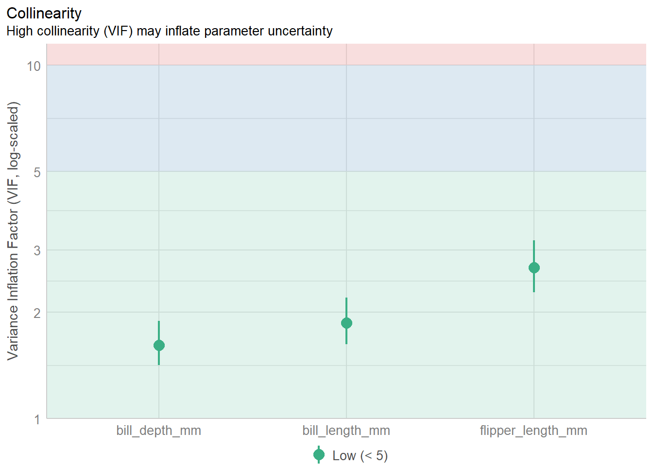

• Solution: use variable selection to delete some X variables.
• Alternatively, use dimension reduction techniques such as Principal Components (Chapter 14).