18.10 Post MICE data management

Sometimes you’ll have a need to do additional data management after imputation has been completed. Creating binary indicators of an event, re-creating scale variables etc. The general approach is to transform the imputed data into long format using complete with the argument include=TRUE , do the necessary data management, and then convert it back to a mids object type.

Continuing with the penguin example, let’s create a new variable that is the ratio of bill length to depth.

Recapping prior steps of imputing, and then creating the completed long data set.

## imp_pen <- mice(pen.miss, m=10, maxit=25, meth="pmm", seed=500, printFlag=FALSE)
pen_long <- complete(imp_pen, 'long', include=TRUE)

We create the new ratio variable on the long data:

pen_long$ratio <- pen_long$bill_length_mm / pen_long$bill_depth_mm

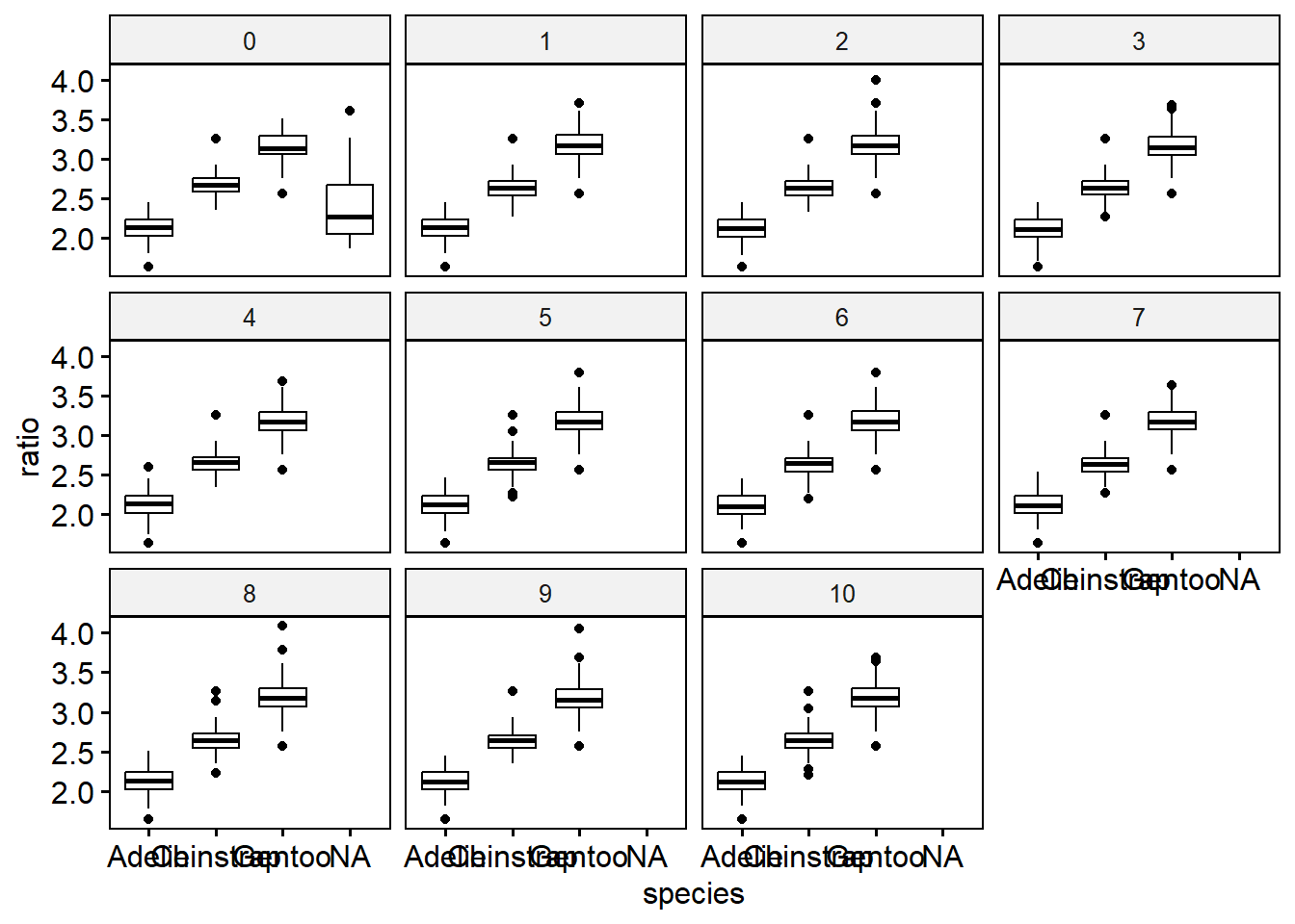
Let’s visualize this to see how different the distributions are across imputation. Notice imputation “0” still has missing data - this is a result of using include = TRUE and keeping the original data as part of the pen_long data.

ggboxplot(pen_long, y="ratio", x="species", facet.by = ".imp")

Then convert the data back to mids object, specifying the variable name that identifies the imputation number.

imp_pen1 <- as.mids(pen_long, .imp = ".imp")

Now we can conduct analyses such as an ANOVA (in linear model form) to see if this ratio differs significantly across the species.

nova.ratio <- with(imp_pen1, lm(ratio ~ species))
pool(nova.ratio) |> summary()
##               term  estimate  std.error statistic       df       p.value
## 1      (Intercept) 2.1221949 0.01435687 147.81738 281.7994 4.610006e-269
## 2 speciesChinstrap 0.5217842 0.02569344  20.30807 245.0315  1.958440e-54
## 3    speciesGentoo 1.0643029 0.02165568  49.14659 254.5258 6.526634e-132