12.2 Distribution of Predicted probabilities

We know that not everyone in the data set is 44.4 years old and makes $20.6k annually (thankfully). So what if you want to get the model predicted probability of the event for all individuals in the data set? There’s no way I’m doing that calculation for every person in the data set.

We can use the predict() command to generate a vector of predictions \(\hat{p}_{i}\) for each row used in the model.

phat.depr <- predict(dep_sex_model, type='response') # create prediction vector
summary(phat.depr)
##    Min. 1st Qu.  Median    Mean 3rd Qu.    Max. 
## 0.01271 0.08352 0.16303 0.17007 0.23145 0.45082
hist(phat.depr) # base R histogram
abline(v = mean(phat.depr), col = "blue", lwd = 2) # add mean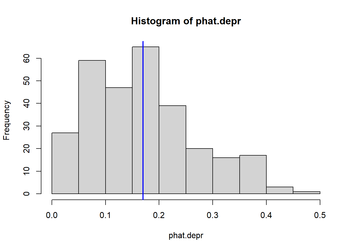

The average predicted probability of showing symptoms of depression is 0.17.

12.2.1 Plotting predictions against covariates

Another important feature to look at is to see how well the model discriminates between the two groups in terms of predicted probabilities. Let’s look at a plot:

Any row with missing data on any variable used in the model will be dropped, and so NOT get a predicted value. So the tactic is to use the data stored in the model object.

model.pred.data <- cbind(dep_sex_model$data, phat.depr)
tail(names(model.pred.data))
## [1] "regdoc"    "treat"     "beddays"   "acuteill"  "chronill"  "phat.depr"

Now that the predictions have been added back onto the data used in the model using cbind, we have covariates to use to plot the predictions against.

ggpubr::ggdensity(model.pred.data, x="phat.depr", add="mean", rug = TRUE, 
          color = "sex", fill = "sex", palette = c("#00AFBB", "#E7B800"))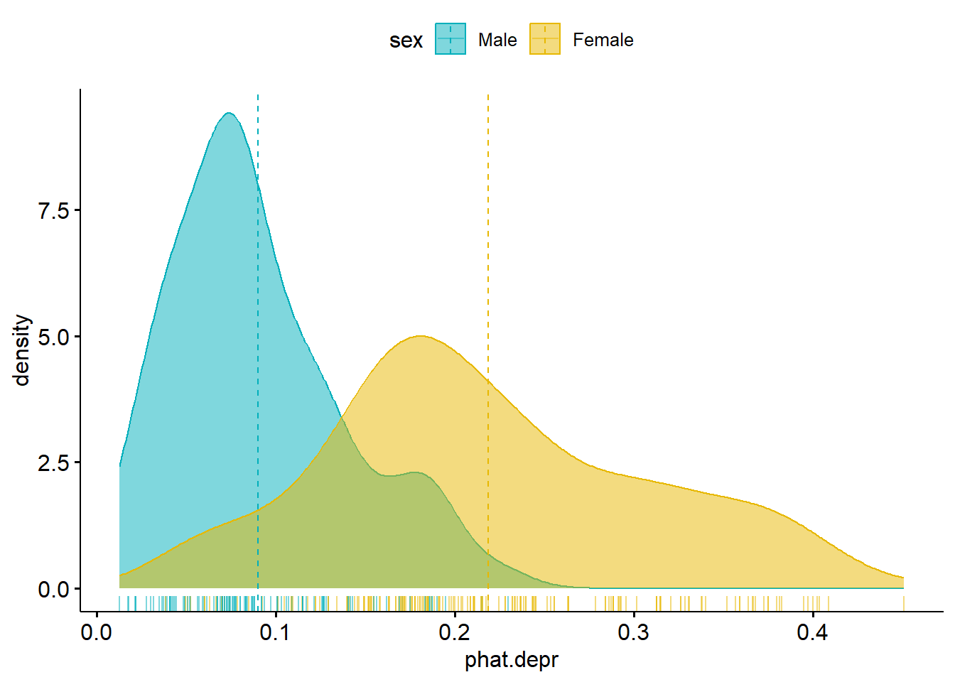

• What do you notice in this plot?
• What can you infer?