7.5 Example

Returning to the Lung function data set from PMA6, lets analyze the relationship between height and FEV for fathers in this data set.

ggplot(fev, aes(y=FFEV1, x=FHEIGHT)) + geom_point() + 
      xlab("Height") + ylab("FEV1") + 
      ggtitle("Scatter Diagram with Regression (blue) and Lowess (red) Lines 
      of FEV1 Versus Height for Fathers.") + 
      geom_smooth(method="lm", se=FALSE, col="blue") + 
      geom_smooth(se=FALSE, col="red")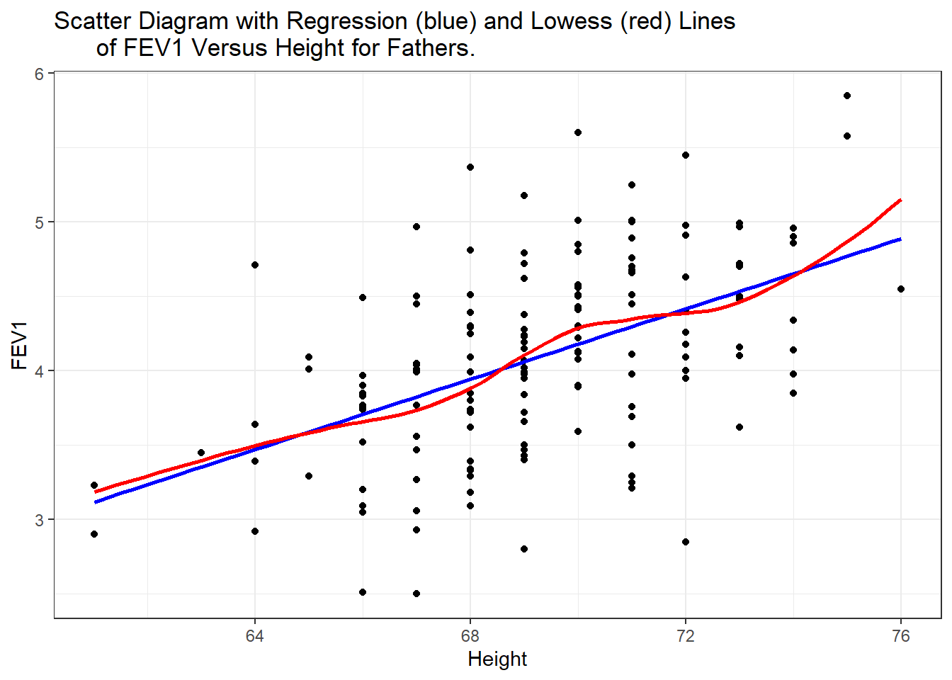 

There does appear to be a tendency for taller men to have higher FEV1. The trend is linear, the red lowess trend line follows the blue linear fit line quite well.

Let’s fit a linear model and report the regression parameter estimates.

fev.dad.model <- lm(FFEV1 ~ FHEIGHT, data=fev)
broom::tidy(fev.dad.model) |> kable(digits=3)

term	estimate	std.error	statistic	p.value
(Intercept)	-4.087	1.152	-3.548	0.001
FHEIGHT	0.118	0.017	7.106	0.000

The least squares equation is \(Y = -4.09 + 0.118X\). We can calculate the confidence interval for that estimate using the confint function.

confint(fev.dad.model) |> kable(digits=3)

	2.5 %	97.5 %
(Intercept)	-6.363	-1.810
FHEIGHT	0.085	0.151

For ever inch taller a father is, his FEV1 measurement significantly increases by .12 (95%CI: .09, .15, p<.0001).