17.1 Pooling
To highlight the benefits of random intercepts models we will compare three linear regression models:
- complete pooling
- no pooling
- partial pooling (the random intercept model)
Complete Pooling
The complete pooling model pools all counties together to give one single estimate of the \(log(radon)\) level.
No Pooling
No pooling refers to the fact that no information is shared among the counties. Each county is independent of the next.
Partial Pooling
The partial pooling model, partially shares information among the counties.
Each county should get a unique intercept such that the collection of county intercepts are randomly sampled from a normal distribution with mean \(0\) and variance \(\sigma^2_{\alpha}\).
Because all county intercepts are randomly sampled from the same theoretical population, \(N(0, \sigma^2_{\alpha})\), information is shared among the counties. This sharing of information is generally referred to as shrinkage, and should be thought of as a means to reduce variation in estimates among the counties. When a county has little information to offer, it’s estimated intercept will be shrunk towards to overall mean of all counties.
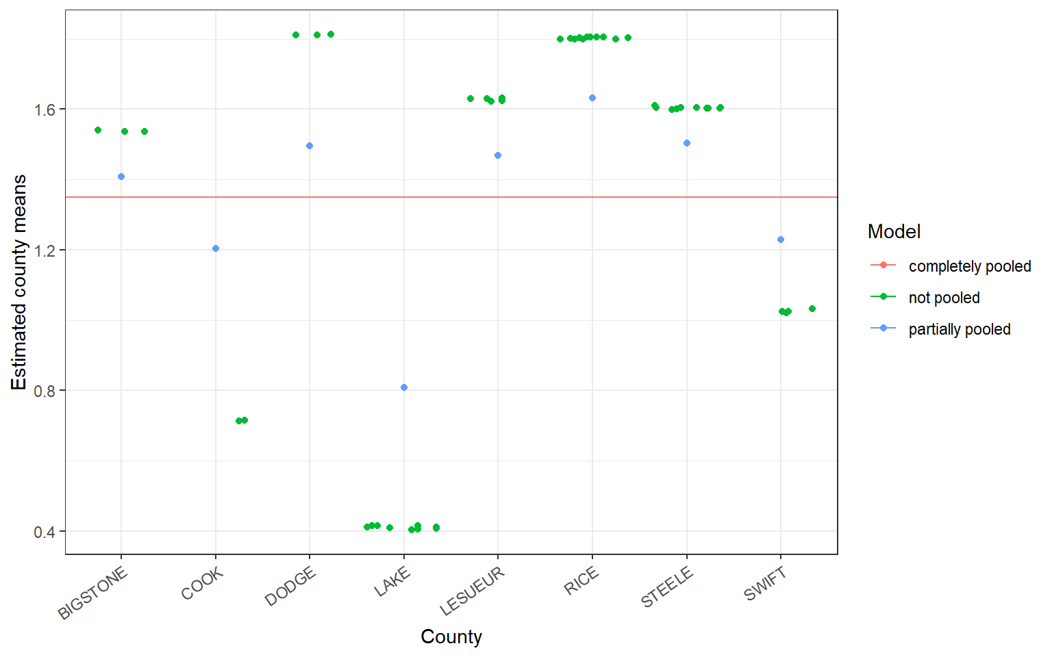
The plot below displays the overall mean as the complete pooling estimate (solid, horizontal line), the no pooling and partial pooling estimates for 8 randomly selected counties contained in the radon data. The amount of shrinkage from the partial pooling fit is determined by a data dependent compromise between the county level sample size, the variation among the counties, and the variation within the counties.

Generally, we can see that counties with smaller sample sizes are shrunk more towards the overall mean, while counties with larger sample sizes are shrunk less.
The fitted values corresponding to different observations within each county of the no-pooling model are jittered to help the eye determine approximate sample size within each county.
Estimates of variation within each county should not be determined from this arbitrary jittering of points.