7.7 Prediction

The predict function is used to create model based predictions.

7.7.1 Predict the average value of Y (\(\hat{y}\)) based on the model

Create predictions for all observations in the data based on the model, and then take the mean of those \(n\) predictions.

\[ \hat{y_{i}} = b_{0} + b_{1}x_{i} \\ \hat{\mu} = \frac{1}{n}\hat{y_{i}} \]

predict(fev.dad.model) |> mean()
## [1] 4.093267

7.7.2 Confidence intervals for the predicted mean

We can leverage the t.test() function to give us the confidence interval for \(\hat{\mu}\)

t.test(predict(fev.dad.model))
## 
##  One Sample t-test
## 
## data:  predict(fev.dad.model)
## t = 152.73, df = 149, p-value < 2.2e-16
## alternative hypothesis: true mean is not equal to 0
## 95 percent confidence interval:
##  4.040309 4.146225
## sample estimates:
## mean of x 
##  4.093267

This model predicts that fathers will have FEV1 measurements of 4.09 (95% CI 4.04, 4.14) on average.

7.7.3 Predict the average value of Y \((\hat{y_{i}})\) for a certain value of \(x^{*}\)

This is also called the fitted value.

\[\hat{y_{i}} = b_{0} + b_{1}x^{*}_{i}\]

We create a new data.frame that holds the values of the data we want to predict. \(x^{*}=60\) in the first example, \(x^{*}=65\) and \(68\) in the second example.

predict(fev.dad.model, newdata = data.frame(FHEIGHT = 60))
##        1 
## 2.999612
predict(fev.dad.model, newdata = data.frame(FHEIGHT = c(65, 68)))
##        1        2 
## 3.590138 3.944454

The confidence interval for the fitted value \(\hat{y_{i}}\) is

\[ \hat{Y} \pm t_{\frac{\alpha}{2}}S \bigg[ \frac{1}{N} + \sqrt{\frac{(X^* - \bar{X})^{2}}{\sum(X - \bar{X})^{2}}} \quad \bigg] \]

where \(S\) is the sample estimated variance (RMSE). We can use the interval argument to predict to calculate this interval.

predict(fev.dad.model, 
        newdata = data.frame(FHEIGHT = c(65, 68)),
        interval = "confidence")
##        fit      lwr      upr
## 1 3.590138 3.423257 3.757019
## 2 3.944454 3.844515 4.044393

7.7.4 Predict a new value of Y \(\hat{y_{i}}\) for a certain value of \(x^{*}\)

The point estimate of \(\hat{y_{i}}\) is calculated the same, but the prediction interval is wider. This is because individual \(y\)’s are more variable than the average. This is the same concept that we saw when studying sampling distributions. The standard deviation of the mean \(\mu_{Y}\), is smaller than the standard deviation of the individual data points \(y_{i}\).

\[ \hat{Y} \pm t_{\frac{\alpha}{2}}S \bigg[ 1+ \frac{1}{N} + \sqrt{\frac{(X^* - \bar{X})^{2}}{\sum(X - \bar{X})^{2}}} \quad \bigg] \]

This is obtained in R by modifying the value of the interval argument.

predict(fev.dad.model, 
        newdata = data.frame(FHEIGHT = c(65, 68)),
        interval = "prediction")
##        fit      lwr      upr
## 1 3.590138 2.463568 4.716709
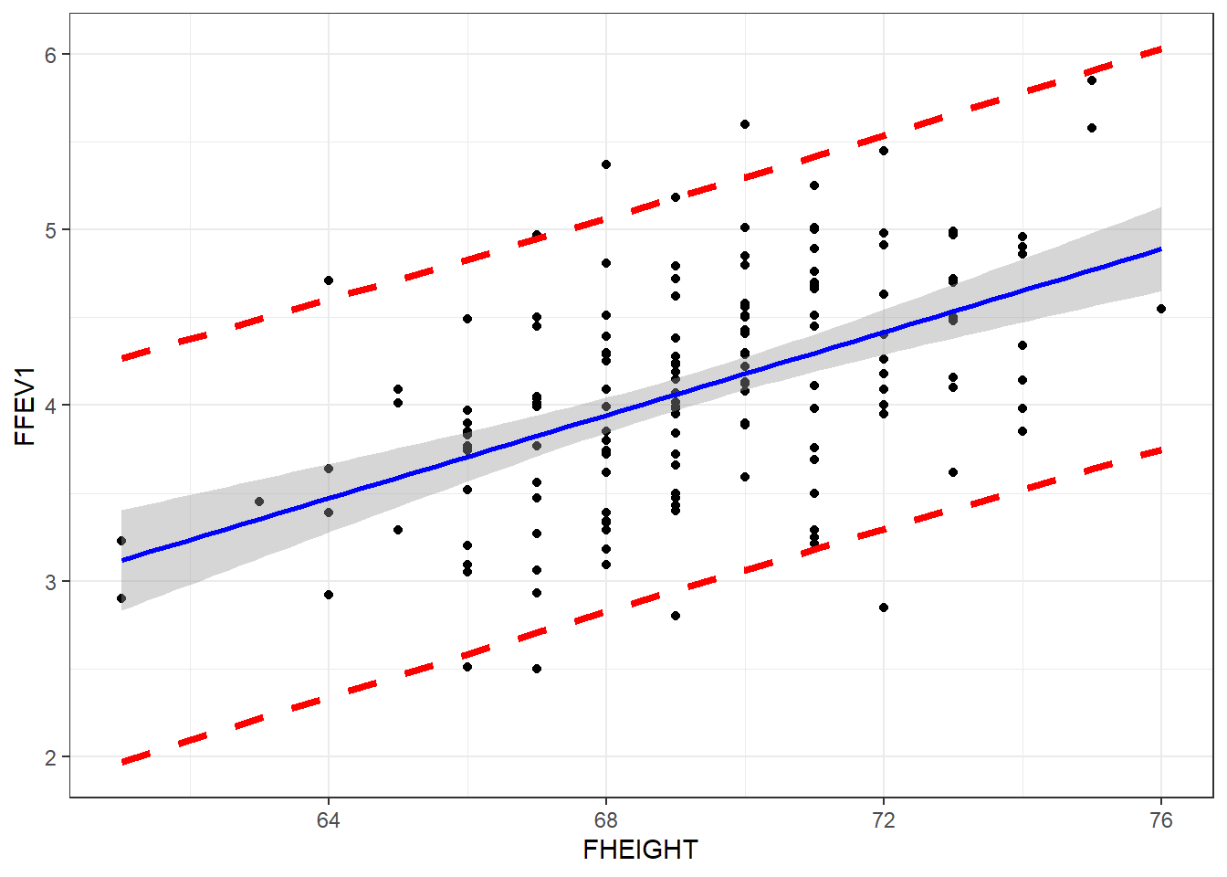
## 2 3.944454 2.825839 5.063069

If we set the se argument in geom_smooth to TRUE, the shaded region is the confidence band for the mean. To get the prediction interval, we have use the predict function to calculate the prediction interval, and then we can add that onto the plot as additional geom_lines.

pred.int <- predict(fev.dad.model, interval="predict") |> data.frame()

ggplot(fev, aes(y=FFEV1, x=FHEIGHT)) + geom_point() + 
      geom_smooth(method="lm", se=TRUE, col="blue") + 
      geom_line(aes(y=pred.int$lwr), linetype="dashed", col="red", lwd=1.5) + 
      geom_line(aes(y=pred.int$upr), linetype="dashed", col="red", lwd=1.5)