14.7 Example
This example follows Analysis of depression data set section in PMA6 Section 14.5. This survey asks 20 questions on emotional states that relate to depression. The data is recorded as numeric, but are categorical in nature where 0 - “rarely or none of the time”, 1 - “some or a little of the time” and so forth.
depress <- read.delim("https://norcalbiostat.netlify.com/data/depress_081217.txt", header=TRUE)
table(depress$c1)
##
##   0   1   2   3
## 225  43  14  12
These questions are typical of what is asked in survey research, and often are thought of, or treated as pseudo-continuous. They are ordinal categorical variables, but they are not truly interval measures since the “distance” between 0 and 1 (rarely and some of the time), would not be considered the same as the distance between 2 (moderately) and 3 (most or all of the time). And “moderately” wouldn’t be necessarily considered as “twice” the amount of “rarely”.
Our options to use these ordinal variables in a model come down to three options.
- convert to a factor and include it as a categorical (series of indicators) variable.
- This can be even more problematic when there are 20 categorical variables. You run out of degrees of freedom very fast with that many predictors.
- leave it as numeric and treat it as pseudo-continuous ordinal measure. Where you can interpret as “as x increases y changes by…”, but
- aggregate across multiple likert-type-ordinal variables and create a new calculated scale variable that can be treated as continuous.
- This is what PCA does by creating new variables \(C_{1}\) that are linear combinations of the original \(x's\).
In this example I use PCA to reduce these 20 correlated variables down to a few uncorrelated variables that explain the most variance.
1. Read in the data and run princomp on the C1:C20 variables.
pc_dep  <- princomp(depress[,9:28], cor=TRUE)
summary(pc_dep)
## Importance of components:
##                           Comp.1     Comp.2     Comp.3     Comp.4     Comp.5
## Standard deviation     2.6562036 1.21883931 1.10973409 1.03232021 1.00629648
## Proportion of Variance 0.3527709 0.07427846 0.06157549 0.05328425 0.05063163
## Cumulative Proportion  0.3527709 0.42704935 0.48862483 0.54190909 0.59254072
##                            Comp.6     Comp.7     Comp.8     Comp.9    Comp.10
## Standard deviation     0.98359581 0.97304489 0.87706188 0.83344885 0.81248191
## Proportion of Variance 0.04837304 0.04734082 0.03846188 0.03473185 0.03300634
## Cumulative Proportion  0.64091375 0.68825457 0.72671645 0.76144830 0.79445464
##                           Comp.11    Comp.12    Comp.13    Comp.14    Comp.15
## Standard deviation     0.77950975 0.74117295 0.73255278 0.71324438 0.67149280
## Proportion of Variance 0.03038177 0.02746687 0.02683168 0.02543588 0.02254513
## Cumulative Proportion  0.82483641 0.85230328 0.87913496 0.90457083 0.92711596
##                           Comp.16    Comp.17    Comp.18    Comp.19     Comp.20
## Standard deviation     0.61252016 0.56673129 0.54273638 0.51804873 0.445396635
## Proportion of Variance 0.01875905 0.01605922 0.01472814 0.01341872 0.009918908
## Cumulative Proportion  0.94587501 0.96193423 0.97666237 0.99008109 1.000000000
2. Pick a subset of PC’s to work with
In the cumulative percentage plot below, I drew a reference line at 80%. So the first 10 PC’s can explain around 80% of the variance in the data.
(create.cumvar.plot <- get_eigenvalue(pc_dep) %>%
  mutate(PC = paste0("PC", 1:20), # create a new variable containing the PC name
         PC = forcats::fct_reorder(PC, cumulative.variance.percent))  # reorder this by the value of the cumulative variance
 )
##        eigenvalue variance.percent cumulative.variance.percent   PC
## Dim.1   7.0554177       35.2770884                    35.27709  PC1
## Dim.2   1.4855693        7.4278463                    42.70493  PC2
## Dim.3   1.2315098        6.1575488                    48.86248  PC3
## Dim.4   1.0656850        5.3284251                    54.19091  PC4
## Dim.5   1.0126326        5.0631630                    59.25407  PC5
## Dim.6   0.9674607        4.8373036                    64.09138  PC6
## Dim.7   0.9468164        4.7340818                    68.82546  PC7
## Dim.8   0.7692375        3.8461877                    72.67164  PC8
## Dim.9   0.6946370        3.4731850                    76.14483  PC9
## Dim.10  0.6601269        3.3006343                    79.44546 PC10
## Dim.11  0.6076355        3.0381773                    82.48364 PC11
## Dim.12  0.5493373        2.7466867                    85.23033 PC12
## Dim.13  0.5366336        2.6831679                    87.91350 PC13
## Dim.14  0.5087176        2.5435878                    90.45708 PC14
## Dim.15  0.4509026        2.2545129                    92.71160 PC15
## Dim.16  0.3751809        1.8759047                    94.58750 PC16
## Dim.17  0.3211844        1.6059218                    96.19342 PC17
## Dim.18  0.2945628        1.4728139                    97.66624 PC18
## Dim.19  0.2683745        1.3418724                    99.00811 PC19
## Dim.20  0.1983782        0.9918908                   100.00000 PC20

ggplot(create.cumvar.plot,
       aes(y = PC,
           x = cumulative.variance.percent)) +
  geom_point(size=4) +
  geom_vline(xintercept = 80)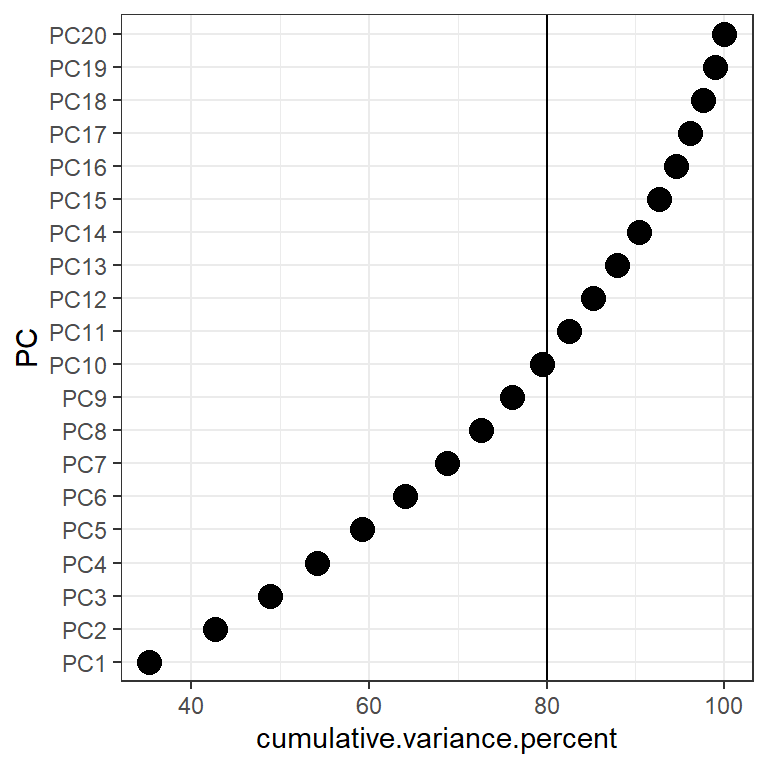
3. Create a Scree plot by plotting the eigenvalue or the proportion of variance from that eigenvalue against the PC number.
gridExtra::grid.arrange(
  fviz_eig(pc_dep, choice = "eigenvalue", addlabels = TRUE),
  fviz_screeplot(pc_dep, addlabels = TRUE)
)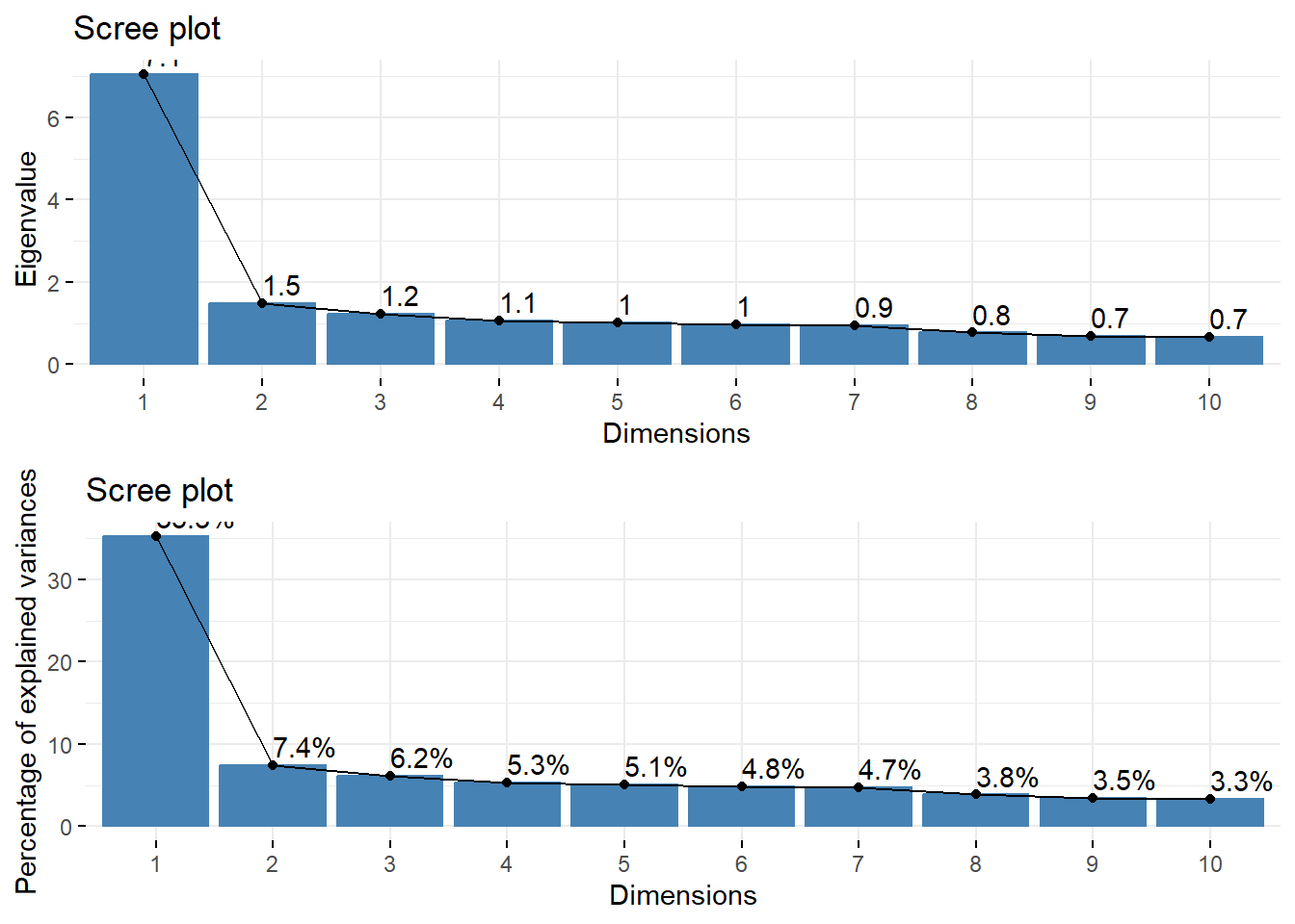
- Option 1: Take all eigenvalues > 1 (\(m=5\))
- Option 2: Use a cutoff point where the lines joining consecutive points are steep to the left of the cutoff point and flat right of the cutoff point. Point where the two slopes meet is the elbow. (\(m=2\)).
4. Examine the loadings
pc_dep$loadings[1:3,1:5]
##       Comp.1      Comp.2     Comp.3       Comp.4      Comp.5
## c1 0.2774384  0.14497938 0.05770239  0.002723687  0.08826773
## c2 0.3131829 -0.02713557 0.03162990 -0.247811083  0.02439748
## c3 0.2677985  0.15471968 0.03459037 -0.247246879 -0.21830547
Here
- \(X_{1}\) = “I felt that I could not shake…”
- \(X_{2}\) = “I felt depressed…”
So the PC’s are calculated as
\[ C_{1} = 0.277x_{1} + 0.313x_{2} + \ldots \\ C_{2} = -0.1449x_{1} + 0.0271x_{2} + \ldots \]
etc…
5. Interpret the PC’s
- Visualize the loadings using
heatmap.2()in thegplotspackage.- I reversed the colors so that red was high positive correlation and yellow/white is low.
- half the options I use below come from this SO post. I had no idea what they did, so I took what the solution showed, and played with it (added/changed some to see what they did), and reviewed
?heatmap.2to see what options were available.
heatmap.2(pc_dep$loadings[,1:5], scale="none", Rowv=NA, Colv=NA, density.info="none",
          dendrogram="none", trace="none", col=rev(heat.colors(256)))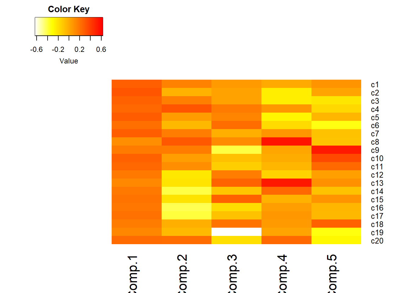
- Loadings over 0.5 (red) help us interpret what these components could “mean”
- Must know exact wording of component questions
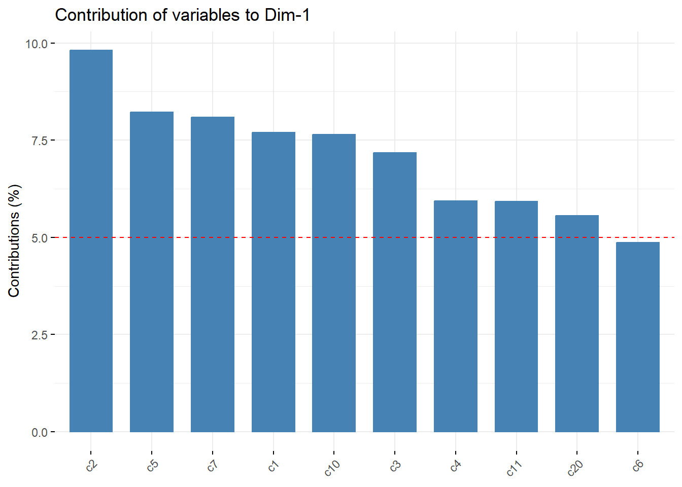
- \(C_{1}\): a weighted average of most items. High value indicates the respondent had many symptoms of depression. Note sign of loadings are all positive and all roughly the same color.
- Recall
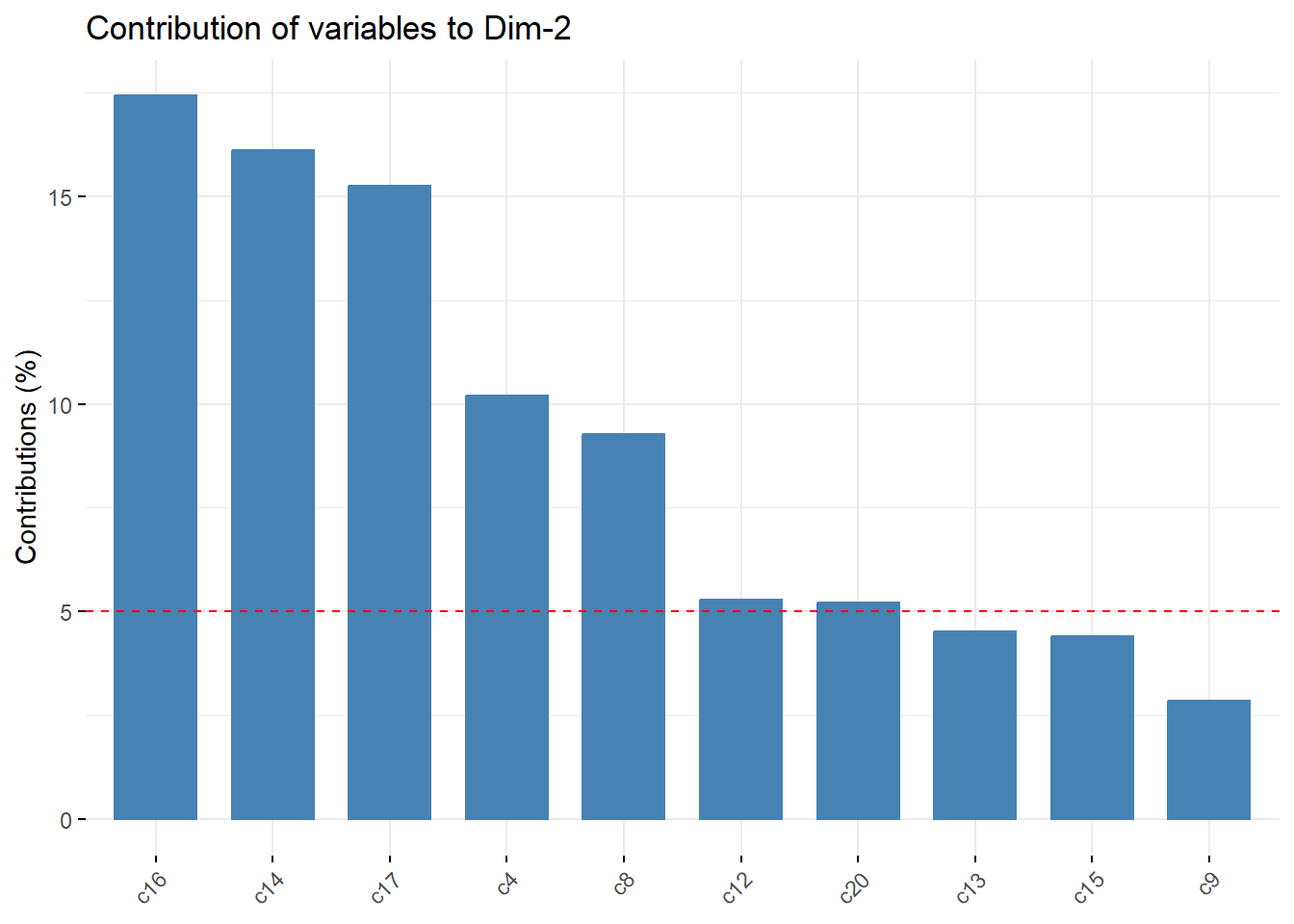
- \(C_{2}\): lethargy (high energetic). High loading on c14, 16, 17, low on 4, 8, 20
- \(C_{3}\): friendliness of others. Large negative loading on c19, c9
etc.
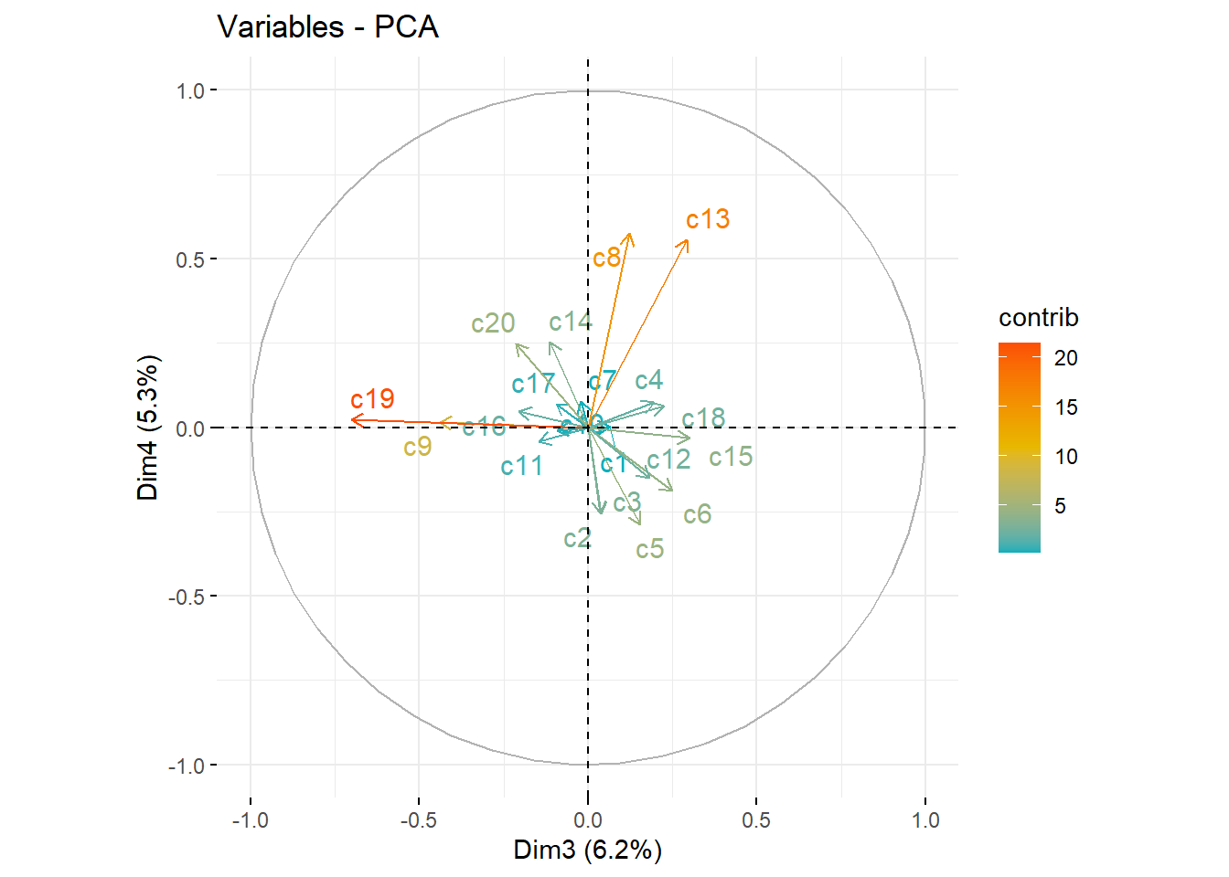
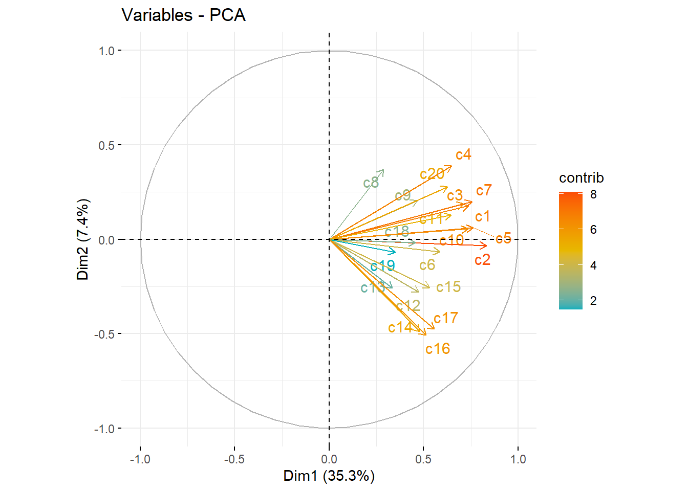
Contributions*
fviz_pca_var(pc_dep, col.var = "contrib", axes=c(1,2),
             gradient.cols = c("#00AFBB", "#E7B800", "#FC4E07"),
             repel = TRUE # Avoid text overlapping
             )
fviz_pca_var(pc_dep, col.var = "contrib", axes=c(3,4),
             gradient.cols = c("#00AFBB", "#E7B800", "#FC4E07"),
             repel = TRUE # Avoid text overlapping
             )