15.5 Rotating Factors
- Find new factors that are easier to interpret
- For each \(X\), we want some high/large (near 1) loadings and some low/small (near zero)
- Two common rotation methods: Varimax rotation, and oblique rotation.
Same(ish) goal as PCA, find a new set of axes to represent the factors.
15.5.1 Varimax Rotation
- Restricts the new axes to be orthogonal to each other. (Factors are independent)
- Maximizes the sum of the variances of the squared factor loadings within each factor \(\sum Var(l_{ij}^{2}|F_{j})\)
- Interpretations slightly less clear
Varimax rotation with principal components extraction.
pc.extract.varimax <- principal(stan.dta, nfactors=2, rotate="varimax")
print(pc.extract.varimax)
## Principal Components Analysis
## Call: principal(r = stan.dta, nfactors = 2, rotate = "varimax")
## Standardized loadings (pattern matrix) based upon correlation matrix
##     RC1   RC2   h2    u2 com
## X1 0.06  0.94 0.89 0.112 1.0
## X2 0.11  0.93 0.89 0.113 1.0
## X3 0.76 -0.10 0.59 0.406 1.0
## X4 0.93  0.16 0.89 0.109 1.1
## X5 0.91  0.28 0.91 0.086 1.2
##
##                        RC1  RC2
## SS loadings           2.30 1.88
## Proportion Var        0.46 0.38
## Cumulative Var        0.46 0.83
## Proportion Explained  0.55 0.45
## Cumulative Proportion 0.55 1.00
##
## Mean item complexity =  1.1
## Test of the hypothesis that 2 components are sufficient.
##
## The root mean square of the residuals (RMSR) is  0.09
##  with the empirical chi square  16.62  with prob <  4.6e-05
##
## Fit based upon off diagonal values = 0.96
Varimax rotation with maximum likelihood extraction. Here i’m using the cutoff argument to only show the values of loadings over 0.3.
ml.extract.varimax <- factanal(stan.dta, factors=2, rotation="varimax")
print(ml.extract.varimax, digits=2, cutoff=.3)
##
## Call:
## factanal(x = stan.dta, factors = 2, rotation = "varimax")
##
## Uniquenesses:
##   X1   X2   X3   X4   X5
## 0.33 0.06 0.72 0.08 0.01
##
## Loadings:
##    Factor1 Factor2
## X1          0.81
## X2          0.97
## X3  0.53
## X4  0.95
## X5  0.96
##
##                Factor1 Factor2
## SS loadings       2.13    1.67
## Proportion Var    0.43    0.33
## Cumulative Var    0.43    0.76
##
## Test of the hypothesis that 2 factors are sufficient.
## The chi square statistic is 0.4 on 1 degree of freedom.
## The p-value is 0.526
Communalities are unchanged after varimax (part of variance due to common factors). This will always be the case for orthogonal (perpendicular) rotations.
15.5.2 Oblique rotation
- Same idea as varimax, but drop the orthogonality requirement
- less restrictions allow for greater flexibility
- Factors are still correlated
- Better interpretation
- Methods:
- quartimax or quartimin minimizes the number of factors needed to explain each variable
- direct oblimin standard method, but results in diminished interpretability of factors
- promax is computationally faster than direct oblimin, so good for very large datasets
pc.extract.quartimin <- principal(stan.dta, nfactors=2, rotate="quartimin")
ml.extract.promax<- factanal(stan.dta, factors=2, rotation="promax")par(mfrow=c(2,3))
plot(pc.extract.norotate, title="PC + norotate")
plot(pc.extract.varimax, title="PC + Varimax")
plot(pc.extract.quartimin, title="PC + quartimin")
load <- ml.extract.norotate$loadings[,1:2]
plot(load, type="n", main="ML + norotate")
text(load, labels=rownames(load))
load <- ml.extract.varimax$loadings[,1:2]
plot(load, type="n", main="ML + Varimax")
text(load, labels=rownames(load))
load <- ml.extract.promax$loadings[,1:2]
plot(load, type="n", main= "ML + Promax")
text(load, labels=rownames(load)) 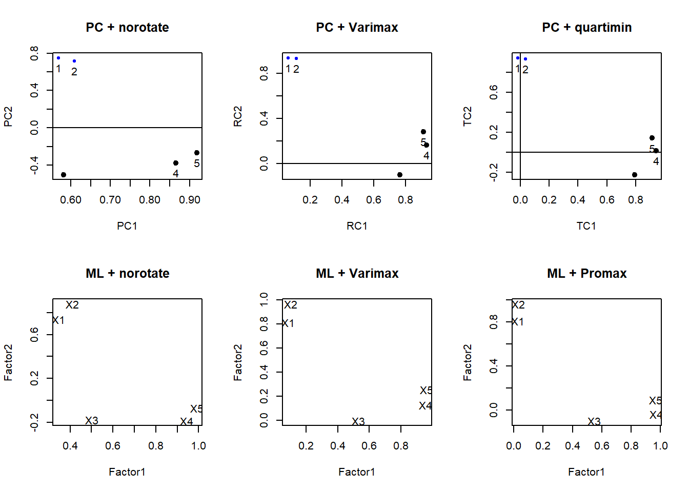
Varimax vs oblique here doesn’t make much of a difference, and typically this is the case. You almost always use some sort of rotation. Recall, this is a hypothetical example and we set up the variables in a distinct two-factor model. So this example will look nice.