8.1 Moderation
Moderation occurs when the relationship between two variables depends on a third variable.
- The third variable is referred to as the moderating variable or simply the moderator.
- The moderator affects the direction and/or strength of the relationship between the explanatory (\(x\)) and response (\(y\)) variable.
- This tends to be an important
- When testing a potential moderator, we are asking the question whether there is an association between two constructs, but separately for different subgroups within the sample.
- This is also called a stratified model, or a subgroup analysis.
8.1.1 Motivating Example - Admissions at UC Berkeley
Sometimes moderating variables can result in what’s known as Simpson’s Paradox. This has had legal consequences in the past at UC Berkeley.
Below are the admissions figures for Fall 1973 at UC Berkeley.
| Applicants | Admitted | |
|---|---|---|
| Total | 12,763 | 41% |
| Men | 8,442 | 44% |
| Women | 4,321 | 35% |
Is there evidence of gender bias in college admissions? Do you think a difference of 35% vs 44% is too large to be by chance?
Department specific data
| All | Men | Women | ||||
| Department | Applicants | Admitted | Applicants | Admitted | Applicants | Admitted |
| A | 933 | 64% | 825 | 62% | 108 | 82% |
| B | 585 | 63% | 560 | 63% | 25 | 68% |
| C | 918 | 35% | 325 | 37% | 593 | 34% |
| D | 792 | 34% | 417 | 33% | 375 | 35% |
| E | 584 | 25% | 191 | 28% | 393 | 24% |
| F | 714 | 6% | 373 | 6% | 341 | 7% |
| Total | 4526 | 39% | 2691 | 45% | 1835 | 30% |
After adjusting for features such as size and competitiveness of the department, the pooled data showed a “small but statistically significant bias in favor of women”
8.1.2 Motivating Example: Association of flower parts
Let’s explore the relationship between the length of the sepal in an iris flower, and the length (cm) of it’s petal.
overall <- ggplot(iris, aes(x=Sepal.Length, y=Petal.Length)) +
                geom_point() + geom_smooth(se=FALSE) +
                theme_bw()

by_spec <- ggplot(iris, aes(x=Sepal.Length, y=Petal.Length, col=Species)) +
                  geom_point() + geom_smooth(se=FALSE) +
                  theme_bw() + theme(legend.position="top")

gridExtra::grid.arrange(overall, by_spec , ncol=2)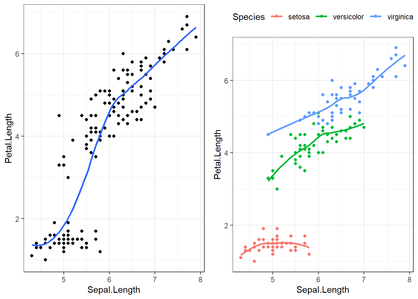
The points are clearly clustered by species, the slope of the lowess line between virginica and versicolor appear similar in strength, whereas the slope of the line for setosa is closer to zero. This would imply that petal length for Setosa may not be affected by the length of the sepal.