18.5 Imputation Methods
This section demonstrates each imputation method on the bsi_depress scale variable from the parental HIV example. To recap, 37% of the data on this variable is missing.
Create an index of row numbers containing missing values. This will be used to fill in those missing values with a data value.
For demonstration purposes I will also create a copy of the bsi_depress variable so that the original is not overwritten for each example.
18.5.1 Unconditional mean substitution.
- Impute all missing data using the mean of observed cases
- Artificially decreases the variance
bsi_depress.ums <- hiv$bsi_depress # copy
complete.case.mean <- mean(hiv$bsi_depress, na.rm=TRUE)
bsi_depress.ums[miss.dep.idx] <- complete.case.mean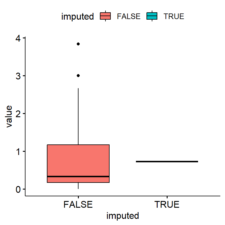
Only a single value was used to impute missing data.
18.5.2 Hot deck imputation
- Impute values by randomly sampling values from observed data.
- Good for categorical data
- Reasonable for MCAR and MAR
- `hotdeck` function in `VIM` availablebsi_depress.hotdeck<- hiv$bsi_depress # copy
hot.deck <- sample(na.omit(hiv$bsi_depress), size = length(miss.dep.idx))
bsi_depress.hotdeck[miss.dep.idx] <- hot.deck
The distribution of imputed values better matches the distribution of observed data, but the distribution (Q1, Q3) is shifted lower a little bit.
18.5.3 Model based imputation
- Conditional Mean imputation: Use regression on observed variables to estimate missing values
- Predictions only available for cases with no missing covariates
- Imputed value is the model predicted mean \(\hat{\mu}_{Y|X}\)
- Could use
VIM::regressionImp()function
- Predictive Mean Matching: Fills in a value randomly by sampling observed values whose regression-predicted values are closest to the regression-predicted value for the missing point.
- Cross between hot-deck and conditional mean
- Categorical data can be imputed using classification models
- Less biased than mean substitution
- but SE’s could be inflated
- Typically used in multivariate imputation (so not shown here)
Model bsi_depress using gender, siblings and age as predictors using linear regression.
reg.model <- lm(bsi_depress ~ gender + siblings + age, hiv)
need.imp  <- hiv[miss.dep.idx, c("gender", "siblings", "age")]
reg.imp.vals <- predict(reg.model, newdata = need.imp)
bsi_depress.lm <- hiv$bsi_depress # copy
bsi_depress.lm[miss.dep.idx] <- reg.imp.vals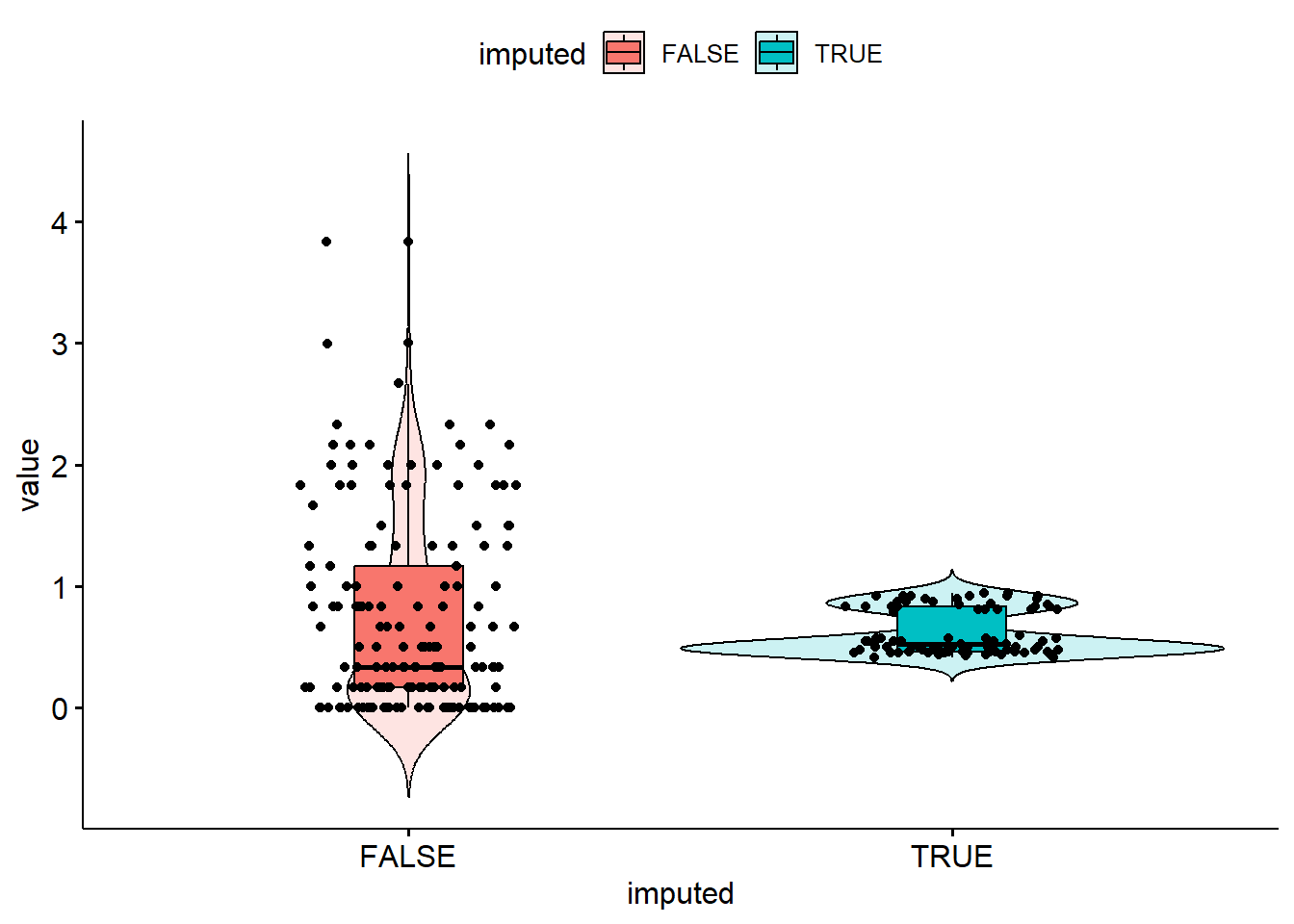
It seems like only values around 0.5 and 0.8 were imputed values for bsi_depress. The imputed values don’t quite match the distribution of observed values. Regression imputation and PMM seem to perform extremely similarily.
18.5.4 Adding a residual
- Impute regression value \(\pm\) a randomly selected residual based on estimated residual variance
- Over the long-term, we can reduce bias, on the average
set.seed(1337)
rmse <- sqrt(summary(reg.model)$sigma)
eps <- rnorm(length(miss.dep.idx), mean=0, sd=rmse)
bsi_depress.lm.resid <- hiv$bsi_depress # copy
bsi_depress.lm.resid[miss.dep.idx] <- reg.imp.vals + eps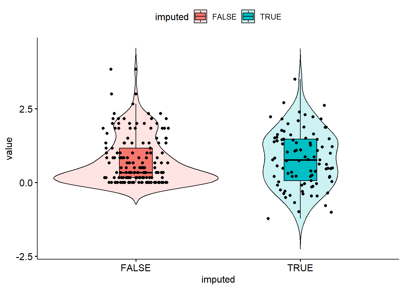
Well, the distribution of imputed values is spread out a bit more, but the imputations do not respect the truncation at 0 this bsi_depress value has.
18.5.5 Comparison of Estimates
Create a table and plot that compares the point estimates and intervals for the average bsi depression scale.
single.imp <- bind_rows(
data.frame(value = na.omit(hiv$bsi_depress),  method = "Observed"),
  data.frame(value = bsi_depress.ums, method = "Mean Sub"),
  data.frame(value = bsi_depress.hotdeck, method = "Hot Deck"),
  data.frame(value = bsi_depress.lm, method = "Regression"),
  data.frame(value = bsi_depress.lm.resid, method = "Reg + eps"))

single.imp$method <- forcats::fct_relevel(single.imp$method ,
      c("Observed", "Mean Sub", "Hot Deck", "Regression", "Reg + eps"))

si.ss <- single.imp %>%
  group_by(method) %>%
  summarize(mean = mean(value),
            sd = sd(value),
            se = sd/sqrt(n()),
            cil = mean-1.96*se,
            ciu = mean+1.96*se)
si.ss
## # A tibble: 5 × 6
##   method      mean    sd     se   cil   ciu
##   <fct>      <dbl> <dbl>  <dbl> <dbl> <dbl>
## 1 Observed   0.723 0.782 0.0622 0.601 0.844
## 2 Mean Sub   0.723 0.620 0.0391 0.646 0.799
## 3 Hot Deck   0.738 0.783 0.0494 0.641 0.835
## 4 Regression 0.682 0.631 0.0399 0.604 0.760
## 5 Reg + eps  0.753 0.848 0.0536 0.648 0.858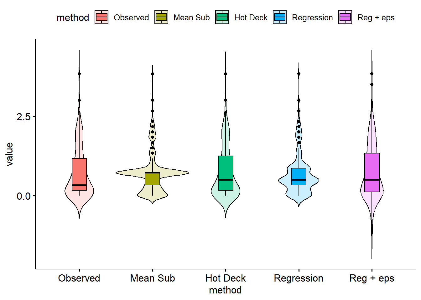
ggplot(si.ss, aes(x=mean, y = method, col=method)) +
  geom_point() + geom_errorbar(aes(xmin=cil, xmax=ciu), width=0.2) +
  scale_x_continuous(limits=c(.5, 1)) +
  theme_bw() + xlab("Average BSI Depression score") + ylab("")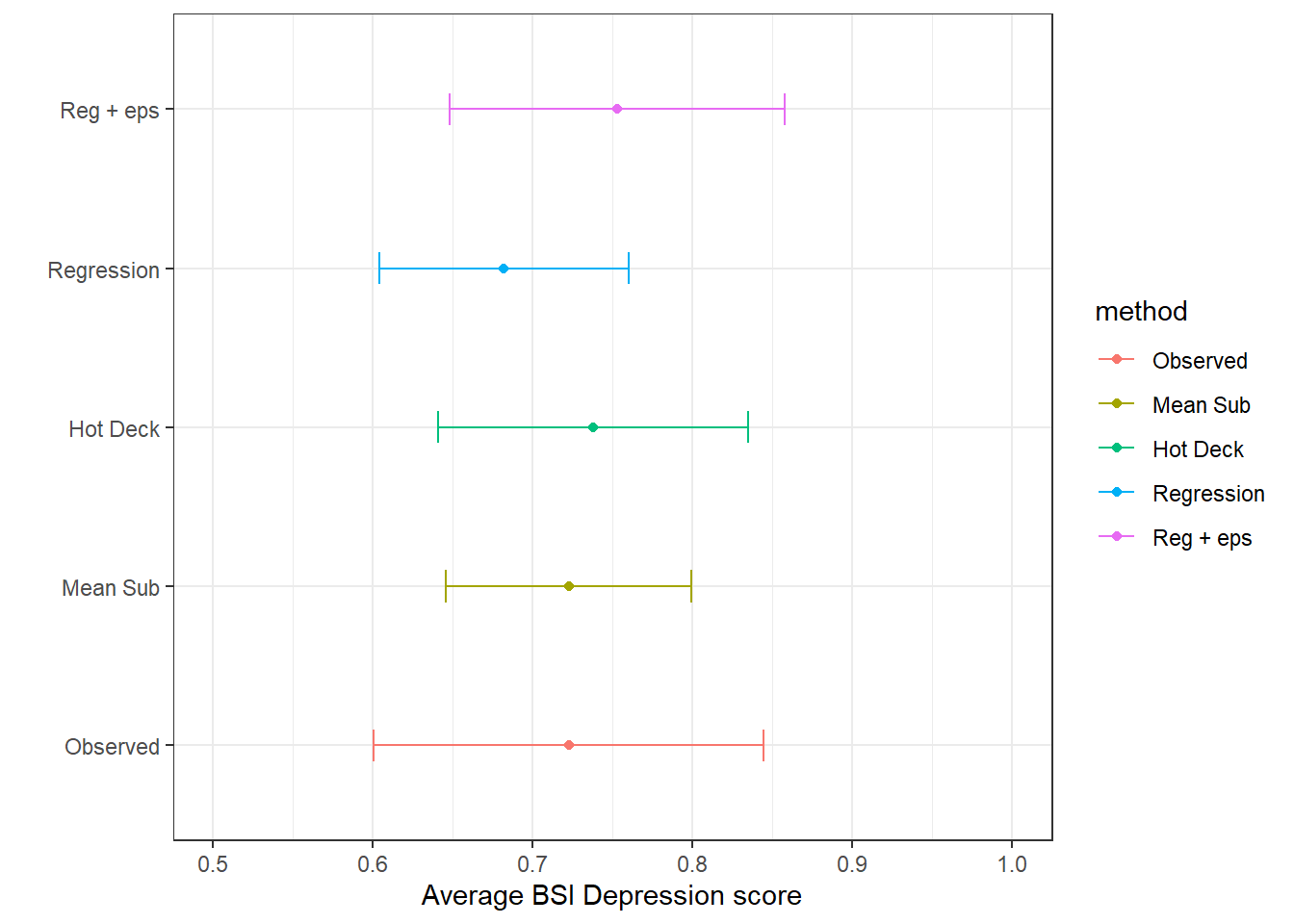
…but we can do better.