18.6 Multiple Imputation (MI)
18.6.1 Goals
- Accurately reflect available information
- Avoid bias in estimates of quantities of interest
- Estimation could involve explicit or implicit model
- Accurately reflect uncertainty due to missingness
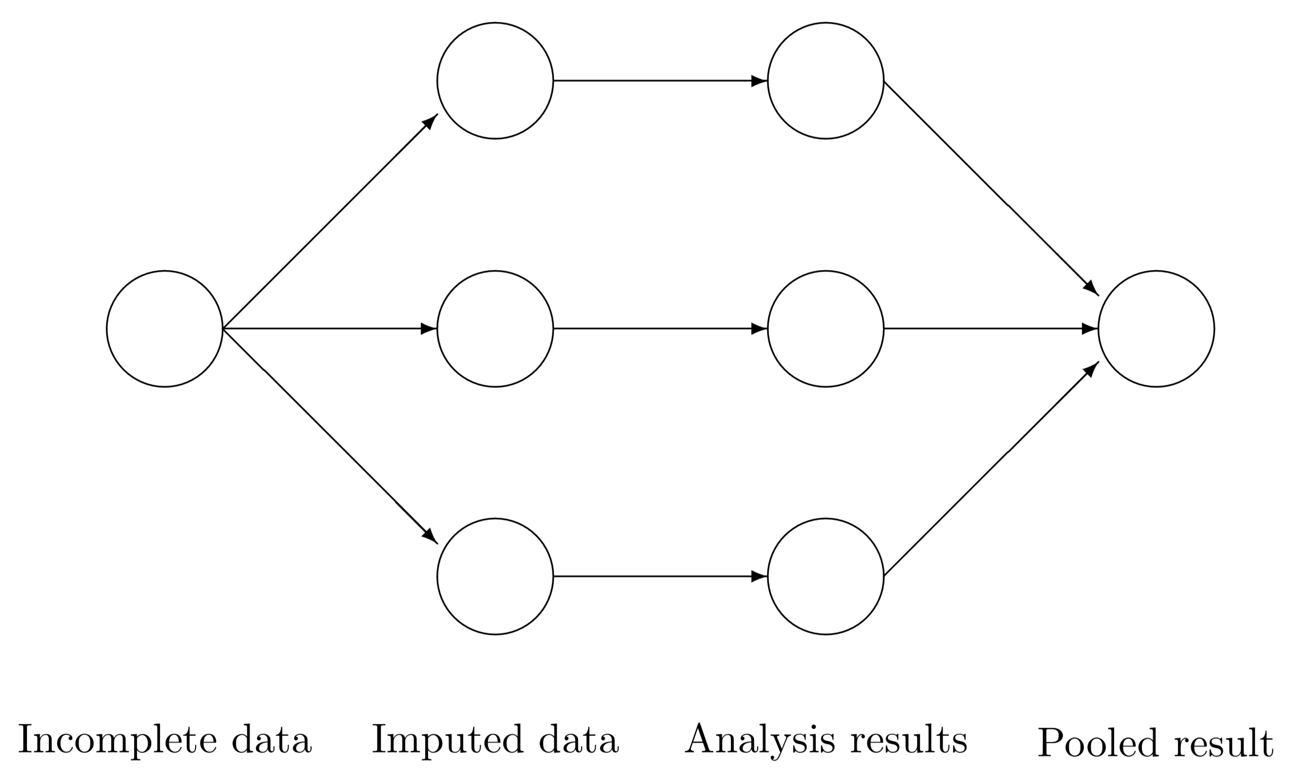
18.6.2 Technique
- For each missing value, impute \(m\) estimates (usually \(m\) = 5)
- Imputation method must include a random component
- Create \(m\) complete data sets
- Perform desired analysis on each of the \(m\) complete data sets
- Pool final estimates in a manner that accounts for the between, and within imputation variance.
18.6.3 MI as a paradigm
- Logic: “Average over” uncertainty, don’t assume most likely scenario (single imputation) covers all plausible scenarios
- Principle: Want nominal 95% intervals to cover targets of estimation 95% of the time
- Simulation studies show that, when MAR assumption holds:
- Proper imputations will yield close to nominal coverage (Rubin 87)
- Improvement over single imputation is meaningful
- Number of imputations can be modest - even 2 adequate for many purposes, so 5 is plenty
Rubin 87: Multiple Imputation for Nonresponse in Surveys, Wiley, 1987).
18.6.4 Inference on MI (Pooling estimates)
Consider \(m\) imputed data sets. For some quantity of interest \(Q\) with squared \(SE = U\), calculate \(Q_{1}, Q_{2}, \ldots, Q_{m}\) and \(U_{1}, U_{2}, \ldots, U_{m}\) (e.g., carry out \(m\) regression analyses, obtain point estimates and SE from each).
Then calculate the average estimate \(\bar{Q}\), the average variance \(\bar{U}\), and the variance of the averages \(B\).
\[ \begin{aligned} \bar{Q} & = \sum^{m}_{i=1}Q_{i}/m \\ \bar{U} & = \sum^{m}_{i=1}U_{i}/m \\ B & = \frac{1}{m-1}\sum^{m}_{i=1}(Q_{i}-\bar{Q})^2 \end{aligned} \]
Then \(T = \bar{U} + \frac{m+1}{m}B\) is the estimated total variance of \(\bar{Q}\).
Significance tests and interval estimates can be based on
\[\frac{\bar{Q}-Q}{\sqrt{T}} \sim t_{df}, \mbox{ where } df = (m-1)(1+\frac{1}{m+1}\frac{\bar{U}}{B})^2\]
- df are similar to those for comparison of normal means with unequal variances, i.e., using Satterthwaite approximation.
- Ratio of (B = between-imputation variance) to (T = between + within-imputation variance) is known as the fraction of missing information (FMI).
- The FMI has been proposed as a way to monitor ongoing data collection and estimate the potential bias resulting from survey non-responders Wagner, 2018
18.6.5 Example
- Create \(m\) imputed datasets using linear regression plus a small amount of random noise so all the imputed values are not identical
set.seed(1061)
dep.imp1 <- dep.imp2 <- dep.imp3 <- regressionImp(bsi_depress ~ gender + siblings + age, hiv)
dep.imp1$bsi_depress[miss.dep.idx] <- dep.imp1$bsi_depress[miss.dep.idx] +
  rnorm(length(miss.dep.idx), mean=0, sd=rmse/2)

dep.imp2$bsi_depress[miss.dep.idx] <- dep.imp2$bsi_depress[miss.dep.idx] +
  rnorm(length(miss.dep.idx), mean=0, sd=rmse/2)

dep.imp3$bsi_depress[miss.dep.idx] <- dep.imp3$bsi_depress[miss.dep.idx] +
  rnorm(length(miss.dep.idx), mean=0, sd=rmse/2)
Visualize the distributions of observed and imputed
dep.mi <- bind_rows(
  data.frame(value = dep.imp1$bsi_depress, imputed = dep.imp1$bsi_depress_imp,
             imp = "dep.imp1"),
  data.frame(value = dep.imp2$bsi_depress, imputed = dep.imp2$bsi_depress_imp,
             imp ="dep.imp2"),
  data.frame(value = dep.imp3$bsi_depress, imputed = dep.imp3$bsi_depress_imp,
             imp ="dep.imp3"))

ggdensity(dep.mi, x = "value", color = "imputed", fill = "imputed",
          add = "mean", rug=TRUE, palette = "jco") +
  facet_wrap(~imp, ncol=1)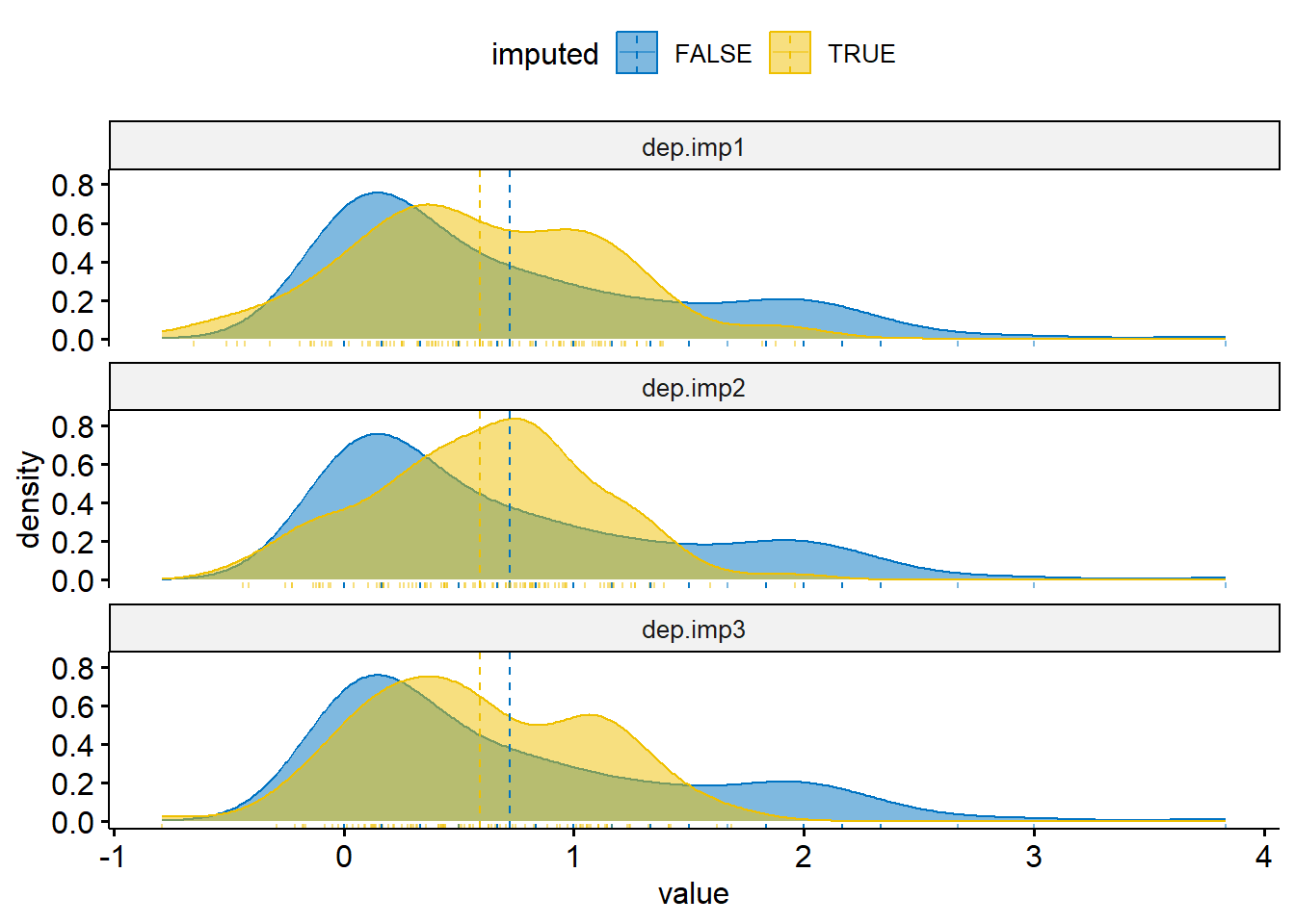
- Calculate the point estimate \(Q\) and the variance \(U\) from each imputation.
(Q <- c(mean(dep.imp1$bsi_depress),
        mean(dep.imp2$bsi_depress),
        mean(dep.imp3$bsi_depress)))
## [1] 0.6700139 0.6808710 0.6694280

n.d <- length(dep.imp1$bsi_depress)
(U <- c(sd(dep.imp1$bsi_depress)/sqrt(n.d),
        sd(dep.imp2$bsi_depress)/sqrt(n.d),
        sd(dep.imp3$bsi_depress)/sqrt(n.d)))
## [1] 0.04443704 0.04324317 0.04365866- Pool estimates and calculate a 95% CI
Q.bar <- mean(Q) # average estimate
U.bar <- mean(U) # average variance
B <- sd(Q) # variance of averages
Tv <- U.bar + ((3+1)/3)*B # Total variance of estimate
df <- 2*(1+(U.bar/(4*B))^2) # degress of freedom
t95 <- qt(.975, df) # critical value for 95% CI
mi.ss <- data.frame(
method = "MI Reg",
mean = Q.bar,
se = sqrt(Tv),
cil = Q.bar - t95*sqrt(Tv),
ciu = Q.bar + t95*sqrt(Tv))
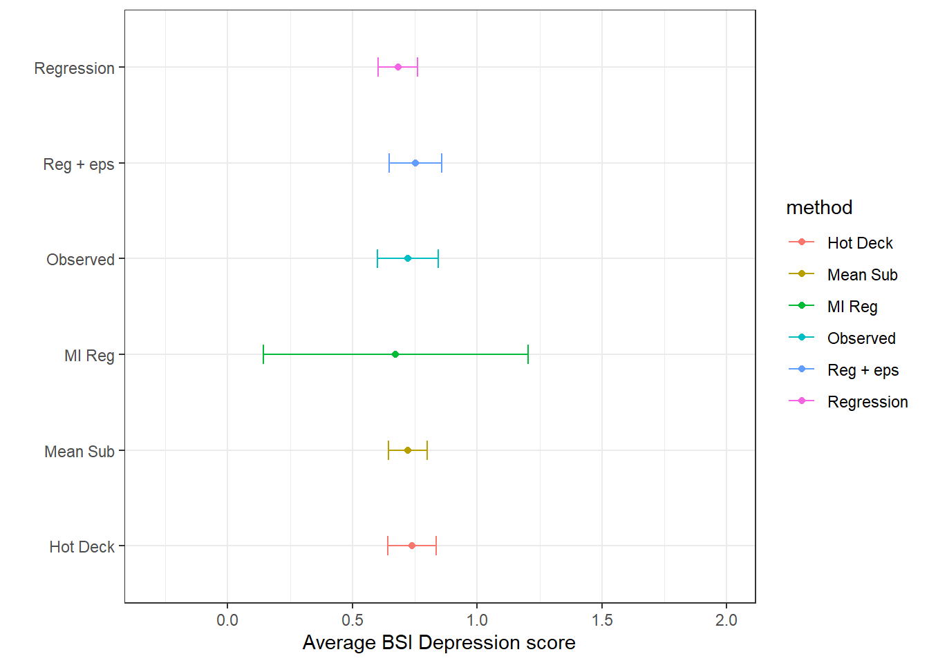
(imp.ss <- bind_rows(si.ss, mi.ss))
## # A tibble: 6 × 6
## method mean sd se cil ciu
## <chr> <dbl> <dbl> <dbl> <dbl> <dbl>
## 1 Observed 0.723 0.782 0.0622 0.601 0.844
## 2 Mean Sub 0.723 0.620 0.0391 0.646 0.799
## 3 Hot Deck 0.738 0.783 0.0494 0.641 0.835
## 4 Regression 0.682 0.631 0.0399 0.604 0.760
## 5 Reg + eps 0.753 0.848 0.0536 0.648 0.858
## 6 MI Reg 0.673 NA 0.229 0.143 1.20ggplot(imp.ss, aes(x=mean, y = method, col=method)) +
geom_point() + geom_errorbar(aes(xmin=cil, xmax=ciu), width=0.2) +
scale_x_continuous(limits=c(-.3, 2)) +
theme_bw() + xlab("Average BSI Depression score") + ylab("")