1.14 Transformations for Normality
Let’s look at assessing normal distributions using the cleaned depression data set.
hist(depress$income, prob=TRUE, xlab="Annual income (in thousands)",
     main="Histogram and Density curve of Income", ylab="")
lines(density(depress$income), col="blue")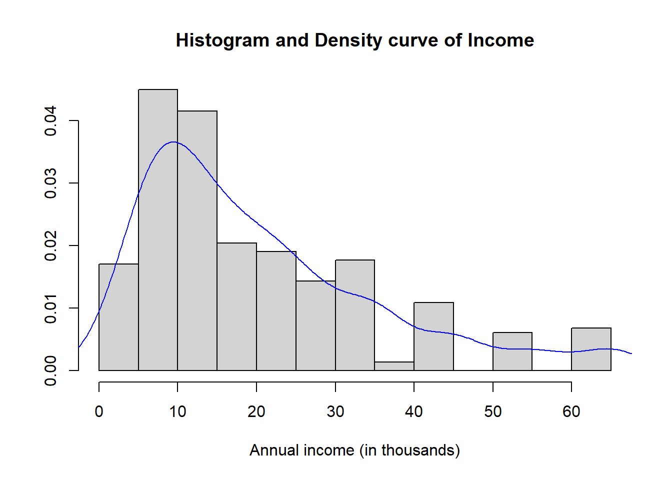
summary(depress$income)
##    Min. 1st Qu.  Median    Mean 3rd Qu.    Max.
##    2.00    9.00   15.00   20.57   28.00   65.00
The distribution of annual income is slightly skewed right with a mean of $20.5k per year and a median of $15k per year income. The range of values goes from $2k to $65k. Reported income above $40k appear to have been rounded to the nearest $10k, because there are noticeable peaks at $40k, $50k, and $60k.
In general, transformations are more effective when the the standard deviation is large relative to the mean. One rule of thumb is if the sd/mean ratio is less than 1/4, a transformation may not be necessary.
Alternatively Hoaglin, Mosteller and Tukey (1985) showed that if the largest observation divided by the smallest observation is over 2, then the data may not be sufficiently variable for the transformation to be decisive.
Note these rules are not meaningful for data without a natural zero.
Another common method of assessing normality is to create a normal probability (or normal quantile) plot.
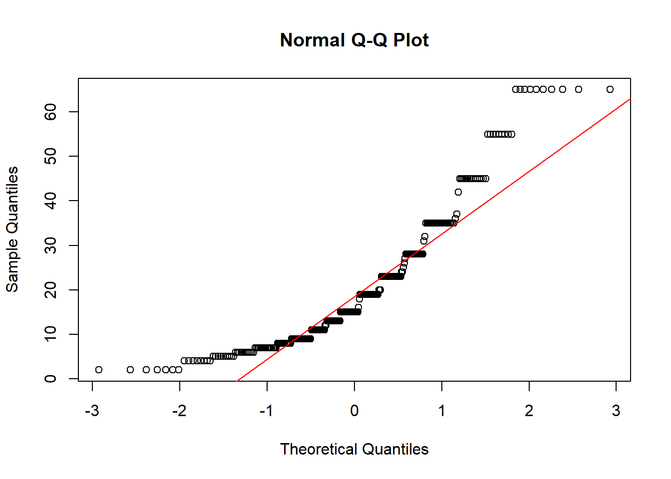
The points on the normal probability plot do not follow the red reference line very well. The dots show a more curved, or U shaped form rather than following a linear line. This is another indication that the data is skewed and a transformation for normality should be created.
- Create three new variables:
log10incas the log base 10 of Income,logincas the natural log of Income, andxincomewhich is equal to the negative of one divided by the cubic root of income.
log10inc <- log10(depress$income)
loginc   <- log(depress$income)
xincome <- -1/(depress$income)^(-1/3)- Create a single plot that display normal probability plots for the original, and each of the three transformations of income. Use the base graphics grid organizer
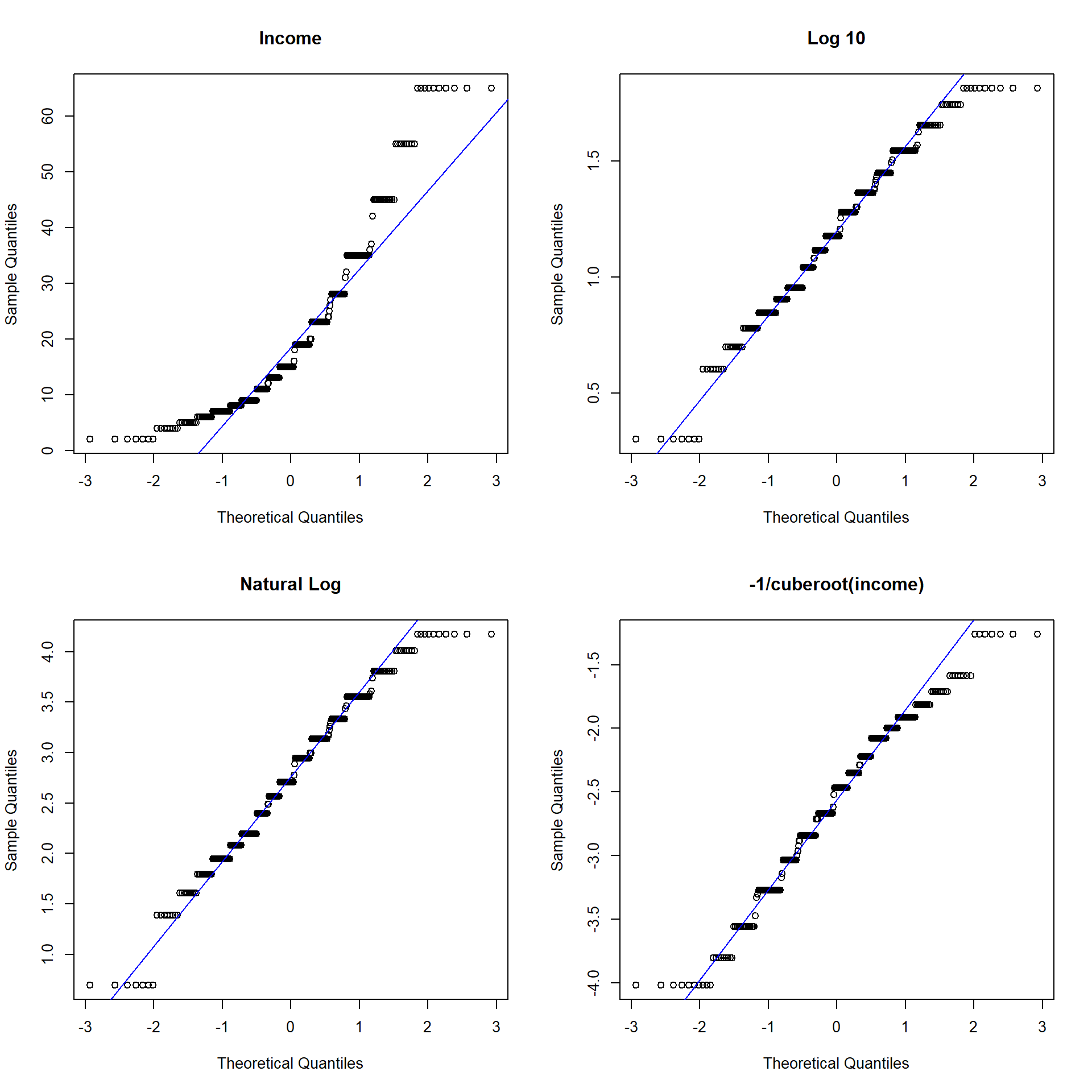
par(mfrow=c(r,c))whereris the number of rows andcis the number of columns. Which transformation does a better job of normalizing the distribution of Income?
par(mfrow=c(2,2)) # Try (4,1) and (1,4) to see how this works.
qqnorm(depress$income, main="Income"); qqline(depress$income,col="blue")
qqnorm(log10inc, main="Log 10"); qqline(log10inc, col="blue")
qqnorm(loginc, main = "Natural Log"); qqline(loginc, col="blue")
qqnorm(xincome, main="-1/cuberoot(income)"); qqline(xincome, col="blue")