5.3 (Q~B) Two means: T-Test

It is common to compare means from different samples. For instance, we might investigate the effectiveness of a certain educational intervention by looking for evidence of greater reading ability in the treatment group against a control group. That is, our research hypothesis is that reading ability of a child is associated with an educational intervention.

The null hypothesis states that there is no relationship, or no effect, of the educational intervention (binary explanatory variable) on the reading ability of the child (quantitative response variable). This can be written in symbols as follows:

$H_{0}: \mu_{1} = \mu_{2}\mbox{ or }\qquad H_{0}: \mu_{1} -\mu_{2}=0$

where $\mu_{1}$ is the average reading score for students in the control group (no intervention) and $\mu_{2}$ be the average reading score for students in the intervention group. Notice it can be written as one mean equals the other, but also as the difference between two means equaling zero. The alternative hypothesis $H_{A}$ states that there is a relationship:

$H_{A}: \mu_{1} \neq \mu_{2} \qquad \mbox{ or } \qquad H_{A}: \mu_{1}-\mu_{2} \neq 0$

5.3.1 Assumptions

The data distribution for each group is approximately normal.
The scores are independent within each group.
The scores from the two groups are independent of each other (i.e. the two samples are independent).

5.3.2 Sampling Distribution for the difference

We use $\bar{x}_1 - \bar{x}_2$ as a point estimate for $\mu_1 - \mu_2$ , which has a standard error of

$SE_{\bar{x}_1 - \bar{x}_2} = \sqrt{SE_{\bar{x}_1}^2 + SE_{\bar{x}_2}^2} = \sqrt{\frac{\sigma^{2}_{1}}{n_1} + \frac{\sigma^{2}_{2}}{n_2}}$

So the equations for a Confidence Interval is,

$\left( \bar{x}_{1} - \bar{x}_{2} \right) \pm t_{\frac{\alpha}{2}, df} \sqrt{ \frac{\sigma^{2}_{1}}{n_{1}} + \frac{\sigma^{2}_{2}}{n_{2}} }$

and Test Statistic is,

$t^{*} = \frac{\left( \bar{x}_{1} - \bar{x}_{2} \right) - d_{0}} {\left( \sqrt{ \frac{\sigma^{2}_{1}}{n_{1}} + \frac{\sigma^{2}_{2}}{n_{2}} } \right )}$

Typically it is unlikely that the population variances $\sigma^{2}_{1}$ and $\sigma^{2}_{2}$ are known so we will use sample variances $s^{2}_{1}$ and $s^{2}_{2}$ as estimates.

While you may never hand calculate these equations, it is important to see the format, or structure, of the equations. Equation $\ref{2sampCImean}$ has the same format of

$\mbox{point estimate} \pm 2*\mbox{standard error}$

regardless what it is we’re actually trying to estimate. Thus in a pinch, you can calculate approximate confidence intervals for whatever estimate you are trying to understand, given only the estimate and standard error, even if the computer program does not give it to you easily or directly.

5.3.3 Example: Smoking and BMI

We would like to know, is there convincing evidence that the average BMI differs between those who have ever smoked a cigarette in their life compared to those who have never smoked? This example uses the Addhealth dataset.

1. Identify response and explanatory variables.

The quantitative response variable is BMI (variable )
The binary explanatory variable is whether the person has ever smoked a cigarette (variable )

2. Visualize and summarize bivariate relationship.

⚠️ Using na.omit() is dangerous! This will remove ALL rows with ANY missing data in it. Regardless if the missing values are contained in the variables you are interested in. The example below employs a trick/work around to not have NA values show in the output. We take the data set addhealth and then select the variables we want to plot, and then we use na.omit() to delete all rows with missing data. Then that is saved as a new, temporary data frame specifically named for this case (plot.bmi.smoke).

note for later. Move this explanation into data viz section.

plot.bmi.smoke <- addhealth %>% select(eversmoke_c, BMI) %>% na.omit()

ggplot(plot.bmi.smoke, aes(x=eversmoke_c, y=BMI, fill=eversmoke_c)) +
      geom_boxplot(width=.3) + geom_violin(alpha=.4) +
      labs(x="Smoking status") +
      scale_fill_viridis_d(guide=FALSE) +
      stat_summary(fun.y="mean", geom="point", size=3, pch=17,
      position=position_dodge(width=0.75))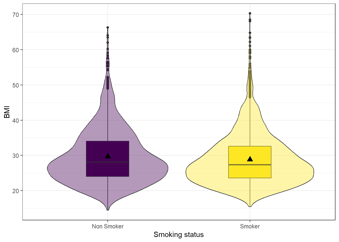

plot.bmi.smoke %>% group_by(eversmoke_c) %>%
 summarise(mean=mean(BMI, na.rm=TRUE),
             sd = sd(BMI, na.rm=TRUE),
             IQR = IQR(BMI, na.rm=TRUE))
## # A tibble: 2 × 4
##   eversmoke_c  mean    sd   IQR
##   <fct>       <dbl> <dbl> <dbl>
## 1 Non Smoker   29.7  7.76  9.98
## 2 Smoker       28.8  7.32  9.02

Smokers have an average BMI of 28.8, smaller than the average BMI of non-smokers at 29.7. Nonsmokers have more variation in their BMIs (sd 7.8 v. 7.3 and IQR 9.98 v. 9.02), but the distributions both look normal, if slightly skewed right.

3. Write the relationship you want to examine in the form of a research question.

Null Hypothesis: There is no relationship between BMI and smoking status.
Alternate Hypothesis: There is a relationship between BMI and smoking status.

4. Perform an appropriate statistical analysis.

I. Let $\mu_1$ denote the average BMI for nonsmokers, and $\mu_2$ the average BMI for smokers.

$\mu_1 - \mu_2 = 0$ There is no difference in the average BMI between smokers and nonsmokers. $\mu_1 - \mu_2 \neq 0$ There is a difference in the average BMI between smokers and nonsmokers.
We are comparing the means between two independent samples. A Two-Sample T-Test for a difference in means will be conducted. The assumptions that the groups are independent is upheld because each individual can only be either a smoker or nonsmoker. The difference in sample means $\bar{x_1} - \bar{x_2}$ is normally distributed – this is a valid assumption due to the large sample size and that differences typically are normally distributed. The observations are independent, and the variability is roughly equal (IQR 9.9 v. 9.0).
We use the t.test function, but use model notation of the format outcome $\sim$ category. Here, BMI is our continuous outcome that we’re testing across the (binary) categorical predictor eversmoke_c.

t.test(BMI ~ eversmoke_c, data=addhealth)
## 
##  Welch Two Sample t-test
## 
## data:  BMI by eversmoke_c
## t = 3.6937, df = 3395.3, p-value = 0.0002245
## alternative hypothesis: true difference in means between group Non Smoker and group Smoker is not equal to 0
## 95 percent confidence interval:
##  0.3906204 1.2744780
## sample estimates:
## mean in group Non Smoker     mean in group Smoker 
##                 29.67977                 28.84722

We have very strong evidence against the null hypothesis, $p = 0.0002$ .

5. Write a conclusion in the context of the problem.

On average, nonsmokers have a significantly higher BMI by 0.83 (0.39, 1.27) compared to nonsmokers ( $p = 0.0002$ ).

⚠️ Always check the output against the direction you are testing. R always will calculate a difference as group 1 - group 2, and it defines the groups alphabetically. For example, for a factor variable that has groups A and B, R will automatically calculate the difference as A-B. In this example it is Nonsmoker - Smoker.