10.1 Interactions (PMA6 8.8)
In this main effects model, Species only changes the intercept. The effect of species is not multiplied by Sepal length. Reviewing the scatterplot below, do you think this is a reasonable model to fit the observed relationship?
ggplot(iris, aes(x=Sepal.Length, y=Petal.Length, color = Species)) +
  geom_point() + geom_smooth(method="lm", se=FALSE)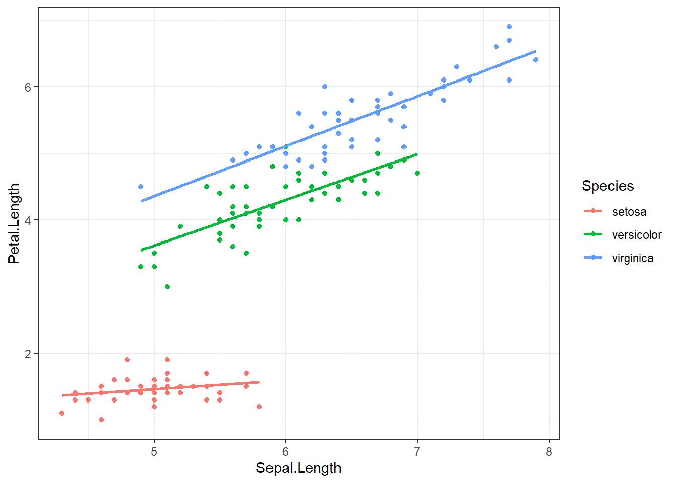
If we care about how species changes the relationship between petal and sepal length, we can fit a model with an interaction between sepal length (\(x_{1}\)) and species. For this first example let \(x_{2}\) be an indicator for when species == setosa. Note that both main effects of sepal length, and setosa species are also included in the model. Interactions are mathematically represented as a multiplication between the two variables that are interacting.
\[ Y_{i} \sim \beta_{0} + \beta_{1}x_{i} + \beta_{2}x_{2i} + \beta_{3}x_{1i}x_{2i}\]
If we evaluate this model for both levels of \(x_{2}\), the resulting models are the same as the stratified models.
When \(x_{2} = 0\), the record is on an iris not from the setosa species.
\[ Y_{i} \sim \beta_{0} + \beta_{1}x_{i} + \beta_{2}(0) + \beta_{3}x_{1i}(0)\] which simplifies to \[ Y_{i} \sim \beta_{0} + \beta_{1}x_{i}\]
When \(x_{2} = 1\), the record is on an iris of the setosa species.
\[ Y_{i} \sim \beta_{0} + \beta_{1}x_{i} + \beta_{2}(1) + \beta_{3}x_{1i}(1)\] which simplifies to \[ Y_{i} \sim (\beta_{0} + \beta_{2}) + (\beta_{1} + \beta_{3})x_{i}\]
Each subgroup model has a different intercept and slope, but we had to estimate 4 parameters in the interaction model, and 6 for the fully stratified model.
10.1.1 Fitting interaction models & interpreting coefficients
Interactions are fit in R by simply multiplying * the two variables together in the model statement.
iris$setosa <- ifelse(iris$Species == "setosa", 1, 0)
lm(Petal.Length ~ Sepal.Length + setosa + Sepal.Length*setosa, data=iris) |> tbl_regression()| Characteristic | Beta | 95% CI1 | p-value |
|---|---|---|---|
| Sepal.Length | 1.0 | 0.91, 1.1 | <0.001 |
| setosa | 2.4 | 0.61, 4.1 | 0.008 |
| Sepal.Length * setosa | -0.90 | -1.2, -0.56 | <0.001 |
| 1 CI = Confidence Interval | |||
The coefficient \(b_{3}\) for the interaction term is significant, confirming that species changes the relationship between sepal length and petal length. Thus, species is a moderator (Chapter 8).
Interpreting Coefficients
- If \(x_{2}=0\), then the effect of \(x_{1}\) on \(Y\) simplifies to: \(\beta_{1}\)
- \(b_{1}\) The effect of sepal length on petal length for non-setosa species of iris (
setosa=0) - For non-setosa species, the petal length increases 1.03cm for every additional cm of sepal length.
- \(b_{1}\) The effect of sepal length on petal length for non-setosa species of iris (
- If \(x_{2}=1\), then the effect of \(x_{1}\) on \(Y\) model simplifies to: \(\beta_{1} + \beta_{3}\)
- For setosa species, the petal length increases by
1.03-0.9=0.13cm for every additional cm of sepal length.
- For setosa species, the petal length increases by
10.1.2 Categorical Interaction variables
Let’s up the game now and look at the full interaction model with a categorical version of species. Recall \(x_{1}\) is Sepal Length, \(x_{2}\) is the indicator for versicolor, and \(x_{3}\) the indicator for virginica . Refer to 9.4.3 for information on how to interpret categorical predictors as main effects.
\[ Y_{i} \sim \beta_{0} + \beta_{1}x_{i} + \beta_{2}x_{2i} + \beta_{3}x_{3i} + \beta_{4}x_{1i}x_{2i} + \beta_{5}x_{1i}x_{3i}+\epsilon_{i}\]
summary(lm(Petal.Length ~ Sepal.Length + Species + Sepal.Length*Species, data=iris))
##
## Call:
## lm(formula = Petal.Length ~ Sepal.Length + Species + Sepal.Length *
##     Species, data = iris)
##
## Residuals:
##      Min       1Q   Median       3Q      Max
## -0.68611 -0.13442 -0.00856  0.15966  0.79607
##
## Coefficients:
##                                Estimate Std. Error t value Pr(>|t|)
## (Intercept)                      0.8031     0.5310   1.512    0.133
## Sepal.Length                     0.1316     0.1058   1.244    0.216
## Speciesversicolor               -0.6179     0.6837  -0.904    0.368
## Speciesvirginica                -0.1926     0.6578  -0.293    0.770
## Sepal.Length:Speciesversicolor   0.5548     0.1281   4.330 2.78e-05 ***
## Sepal.Length:Speciesvirginica    0.6184     0.1210   5.111 1.00e-06 ***
## ---
## Signif. codes:  0 '***' 0.001 '**' 0.01 '*' 0.05 '.' 0.1 ' ' 1
##
## Residual standard error: 0.2611 on 144 degrees of freedom
## Multiple R-squared:  0.9789, Adjusted R-squared:  0.9781
## F-statistic:  1333 on 5 and 144 DF,  p-value: < 2.2e-16
The slope of the relationship between sepal length and petal length is calculated as follows, for each species:
- setosa \((x_{2}=0, x_{3}=0): b_{1}=0.13\)
- versicolor \((x_{2}=1, x_{3}=0): b_{1} + b_{2} + b_{4} = 0.13+0.55 = 0.68\)
- virginica \((x_{2}=0, x_{3}=1): b_{1} + b_{3} + b_{5} = 0.13+0.62 = 0.75\)
Compare this to the estimates gained from the stratified model:
by(iris, iris$Species, function(x){
  lm(Petal.Length ~ Sepal.Length, data=x) %>% coef()
})
## iris$Species: setosa
##  (Intercept) Sepal.Length
##    0.8030518    0.1316317
## ------------------------------------------------------------
## iris$Species: versicolor
##  (Intercept) Sepal.Length
##    0.1851155    0.6864698
## ------------------------------------------------------------
## iris$Species: virginica
##  (Intercept) Sepal.Length
##    0.6104680    0.7500808
They’re the same! Proof that an interaction is equivalent to stratification.
10.1.3 Example 2
What if we now wanted to include other predictors in the model? How does sepal length relate to petal length after controlling for petal width? We add the variable for petal width into the model
summary(lm(Petal.Length ~ Sepal.Length + setosa + Sepal.Length*setosa + Petal.Width, data=iris))
##
## Call:
## lm(formula = Petal.Length ~ Sepal.Length + setosa + Sepal.Length *
##     setosa + Petal.Width, data = iris)
##
## Residuals:
##      Min       1Q   Median       3Q      Max
## -0.83519 -0.18278 -0.01812  0.17004  1.06968
##
## Coefficients:
##                     Estimate Std. Error t value Pr(>|t|)
## (Intercept)         -0.86850    0.27028  -3.213  0.00162 **
## Sepal.Length         0.66181    0.05179  12.779  < 2e-16 ***
## setosa               1.83713    0.62355   2.946  0.00375 **
## Petal.Width          0.97269    0.07970  12.204  < 2e-16 ***
## Sepal.Length:setosa -0.61106    0.12213  -5.003 1.61e-06 ***
## ---
## Signif. codes:  0 '***' 0.001 '**' 0.01 '*' 0.05 '.' 0.1 ' ' 1
##
## Residual standard error: 0.2769 on 145 degrees of freedom
## Multiple R-squared:  0.9761, Adjusted R-squared:  0.9754
## F-statistic:  1478 on 4 and 145 DF,  p-value: < 2.2e-16
So far, petal width, and the combination of species and sepal length are both significantly associated with petal length.
Note of caution: Stratification implies that the stratifying variable interacts with all other variables. So if we were to go back to the stratified model where we fit the model of petal length on sepal length AND petal width, stratified by species, we would be implying that species interacts with both sepal length and petal width.
E.g. the following stratified model
- \(Y = A + B + C + D + C*D\), when D=1
- \(Y = A + B + C + D + C*D\), when D=0
is the same as the following interaction model:
- \(Y = A + B + C + D + A*D + B*D + C*D\)
10.1.4 Example 3:
Let’s explore the relationship between income, employment status and depression. This example follows a logistic regression example from section 11.4.4.
Here I create the binary indicators of lowincome (annual income <$10k/year) and underemployed (part time or unemployed).
depress$lowincome <- ifelse(depress$income < 10, 1, 0)
table(depress$lowincome, depress$income, useNA="always")
##
##         2  4  5  6  7  8  9 11 12 13 15 16 18 19 20 23 24 25 26 27 28 31 32 35
##   0     0  0  0  0  0  0  0 17  2 18 24  1  1 25  3 25  2  1  1  1 19  1  1 24
##   1     7  8 10 12 18 14 22  0  0  0  0  0  0  0  0  0  0  0  0  0  0  0  0  0
##   <NA>  0  0  0  0  0  0  0  0  0  0  0  0  0  0  0  0  0  0  0  0  0  0  0  0
##
##        36 37 42 45 55 65 <NA>
##   0     1  1  1 15  9 10    0
##   1     0  0  0  0  0  0    0
##   <NA>  0  0  0  0  0  0    0

depress$underemployed <- ifelse(depress$employ %in% c("PT", "Unemp"), 1, 0 )
table(depress$underemployed, depress$employ, useNA="always")
##
##         FT Houseperson In School Other  PT Retired Unemp <NA>
##   0    167          27         2     4   0      38     0    0
##   1      0           0         0     0  42       0    14    0
##   <NA>   0           0         0     0   0       0     0    0
The Main Effects model assumes that the effect of income on depression is independent of employment status, and the effect of employment status on depression is independent of income.
me_model <- glm(cases ~ lowincome + underemployed, data=depress, family="binomial")
summary(me_model)
##
## Call:
## glm(formula = cases ~ lowincome + underemployed, family = "binomial",
##     data = depress)
##
## Coefficients:
##               Estimate Std. Error z value Pr(>|z|)
## (Intercept)    -1.9003     0.2221  -8.556  < 2e-16 ***
## lowincome       0.2192     0.3353   0.654  0.51322
## underemployed   1.0094     0.3470   2.909  0.00363 **
## ---
## Signif. codes:  0 '***' 0.001 '**' 0.01 '*' 0.05 '.' 0.1 ' ' 1
##
## (Dispersion parameter for binomial family taken to be 1)
##
##     Null deviance: 268.12  on 293  degrees of freedom
## Residual deviance: 259.93  on 291  degrees of freedom
## AIC: 265.93
##
## Number of Fisher Scoring iterations: 4
To formally test whether an interaction term is necessary, we add the interaction term into the model and assess whether the coefficient for the interaction term is significantly different from zero.
me_intx_model <- glm(cases ~ lowincome + underemployed + lowincome*underemployed, data=depress, family="binomial")
summary(me_intx_model)
##
## Call:
## glm(formula = cases ~ lowincome + underemployed + lowincome *
##     underemployed, family = "binomial", data = depress)
##
## Coefficients:
##                         Estimate Std. Error z value Pr(>|z|)
## (Intercept)              -1.7011     0.2175  -7.822 5.21e-15 ***
## lowincome                -0.4390     0.4324  -1.015  0.31005
## underemployed             0.2840     0.4501   0.631  0.52802
## lowincome:underemployed   2.2615     0.7874   2.872  0.00408 **
## ---
## Signif. codes:  0 '***' 0.001 '**' 0.01 '*' 0.05 '.' 0.1 ' ' 1
##
## (Dispersion parameter for binomial family taken to be 1)
##
##     Null deviance: 268.12  on 293  degrees of freedom
## Residual deviance: 251.17  on 290  degrees of freedom
## AIC: 259.17
##
## Number of Fisher Scoring iterations: 4