15.3 Example data setup
Generate 100 data points from the following multivariate normal distribution:
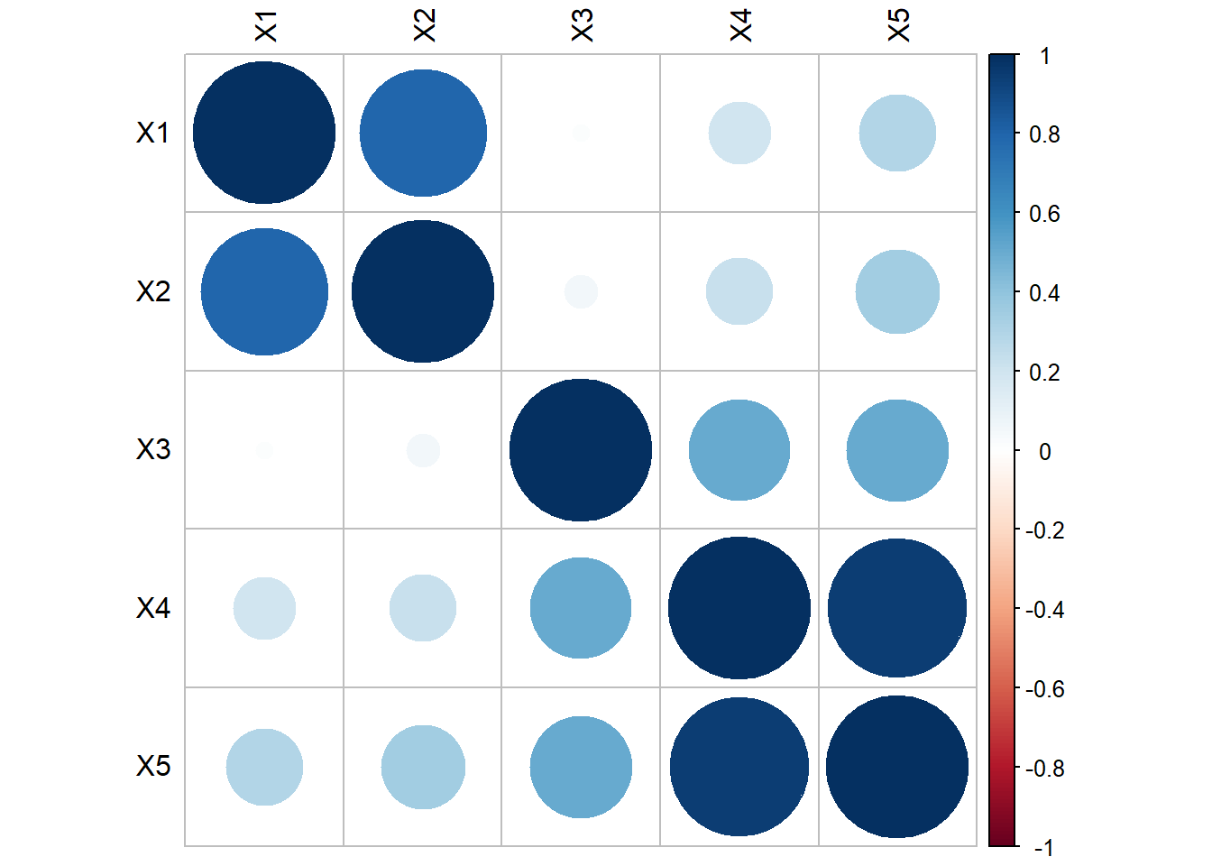
\[\mathbf{\mu} = \left(\begin{array} {r} 0.163 \\ 0.142 \\ 0.098 \\ -0.039 \\ -0.013 \end{array}\right), \mathbf{\Sigma} = \left(\begin{array} {cc} 1 & & & & & \\ 0.757 & 1 & & & & \\ 0.047 & 0.054 & 1 & & & \\ 0.155 & 0.176 & 0.531 & 1 & \\ 0.279 & 0.322 & 0.521 & 0.942 & 1 \end{array}\right) \].
set.seed(456)
m <- c(0.163, 0.142, 0.098, -0.039, -0.013)
s <- matrix(c(1.000, 0.757, 0.047, 0.155, 0.279,
              0.757, 1.000, 0.054, 0.176, 0.322,
              0.047, 0.054, 1.000, 0.531, 0.521,
              0.155, 0.176, 0.531, 1.000, 0.942,
              0.279, 0.322, 0.521, 0.942, 1.000),
            nrow=5)
data <- data.frame(MASS::mvrnorm(n=100, mu=m, Sigma=s))
colnames(data) <- paste0("X", 1:5)
Standardize the \(X\)’s.
The hypothetical data model is that these 5 variables are generated from 2 underlying factors.
\[ \begin{equation} \begin{aligned} X_{1} &= (1)*F_{1} + (0)*F_{2} + e_{1} \\ X_{2} &= (1)*F_{1} + (0)*F_{2} + e_{2} \\ X_{3} &= (0)*F_{1} + (.5)*F_{2} + e_{3} \\ X_{4} &= (0)*F_{1} + (1.5)*F_{2} + e_{4} \\ X_{5} &= (0)*F_{1} + (2)*F_{2} + e_{5} \\ \end{aligned} \end{equation} \]
Implications
- \(F_{1}, F_{2}\) and all \(e_{i}\)’s are independent normal variables
- The first two \(X\)’s are inter-correlated, and the last 3 \(X\)’s are inter-correlated
- The first 2 \(X\)’s are NOT correlated with the last 3 \(X\)’s