11.3 Binary outcome data

Consider an outcome variable \(Y\) with two levels: Y = 1 if event, = 0 if no event.

Let \(p_{i} = P(y_{i}=1)\).

Two goals:

• Assess the impact selected covariates have on the probability of an outcome occurring.
• Predict the probability of an event occurring given a certain covariate pattern. This is covered in section 12

Binary data can be modeled using a Logistic Model or a Probit Model.

The logistic model relates the probability of an event based on a linear combination of X’s.

\[ log\left( \frac{p_{i}}{1-p_{i}} \right) = \beta_{0} + \beta_{1}x_{1i} + \beta_{2}x_{2i} + \ldots + \beta_{p}x_{pi} \]

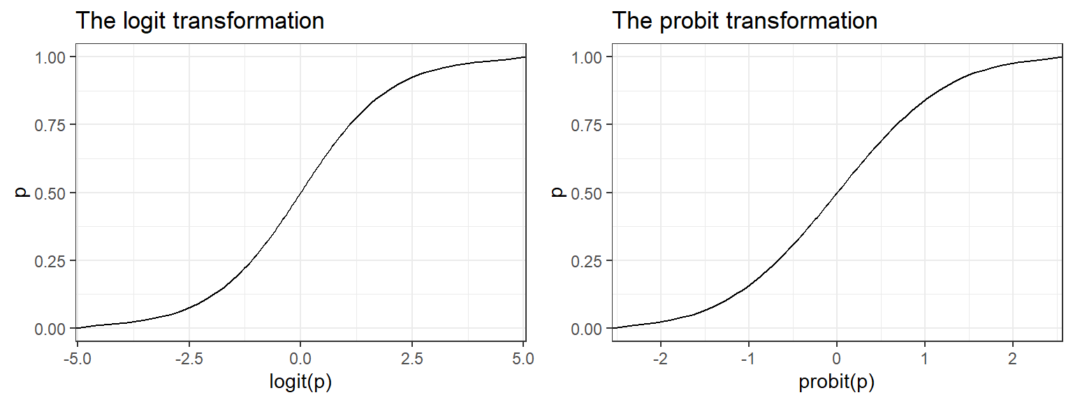
Since the odds are defined as the probability an event occurs divided by the probability it does not occur: \((p/(1-p))\), the function \(log\left(\frac{p_{i}}{1-p_{i}}\right)\) is also known as the log odds, or more commonly called the logit. This is the link function for the logistic regression model.

This in essence takes a binary outcome 0/1 variable, turns it into a continuous probability (which only has a range from 0 to 1) Then the logit(p) has a continuous distribution ranging from \(-\infty\) to \(\infty\), which is the same form as a Multiple Linear Regression (continuous outcome modeled on a set of covariates)

The probit function uses the inverse CDF for the normal distribution as the link function. The effect of the transformation is very similar. For social science interpretation of the coefficients, we tend to choose the logit transformation and conduct a Logistic Regression. For classification purposes, often researchers will test out both transformations to see which one gives the best predictions.