11.2 Log-linear models
A log-linear model is when the log of the response variable is modeled using a linear combination of predictors.
\[ln(Y) \sim XB +\epsilon\]
Recall that in statistics, when we refer to the log, we mean the natural log ln.
This type of model is often use to model count data using the Poisson distribution (Section 11.5).
Why are we transforming the outcome? Typically to achieve normality when the response variable is highly skewed.
Interpreting results
Since we transformed our outcome before performing the regression, we have to back-transform the coefficient before interpretation. Similar to logistic regression, we need to exponentiate the regression coefficient before interpreting.
When using log transformed outcomes, the effect on Y becomes multiplicative instead of additive.
- Additive For every 1 unit increase in X, y increases by b1
- Multiplicative For every 1 unit increase in X, y is multiplied by \(e^{b1}\)
Example, let \(b_{1} = 0.2\).
- Additive For every 1 unit increase in X, y increases by 0.2 units.
- Multiplicative For every 1 unit increase in X, y changes by \(e^{0.2} = 1.22\) = 22%
Thus we interpret the coefficient as a percentage change in \(Y\) for a unit increase in \(x_{j}\).
- \(b_{j}<0\) : Positive slope, positive association. The expected value of \(Y\) for when \(x=0\) is \(1 - e^{b_{j}}\) percent lower than when \(x=1\)
- \(b_{j} \geq 0\) : Negative slope, negative association. The expected value of \(Y\) for when \(x=0\) is \(e^{b_{j}}\) percent higher than when \(x=1\)
This UCLA resource is my “go-to” reference on how to interpret the results when your response, predictor, or both variables are log transformed.
https://stats.idre.ucla.edu/other/mult-pkg/faq/general/faqhow-do-i-interpret-a-regression-model-when-some-variables-are-log-transformed/11.2.1 Example
We are going to analyze personal income from the AddHealth data set. First I need to clean up, and log transform the variable for personal earnings H4EC2 by following the steps below in order.
- Remove values above 999995 (structural missing).
- Create a new variable called
income, that sets all values of personal income to be NA if below the federal poverty line.- First set
income= H4EC2 - Then set income to missing, if
H4EC2 < 10210(the federal poverty limit from 2008)
- First set
- Then create a new variable:
logincomethat is the natural log (ln) of income. e.g.addhealth$logincome = log(addhealth$income)
Why are we transforming income? To achieve normality.
par(mfrow=c(2,2))
hist(addhealth$income, probability = TRUE); lines(density(addhealth$income, na.rm=TRUE), col="red")
hist(addhealth$logincome, probability = TRUE); lines(density(addhealth$logincome, na.rm=TRUE), col="blue")
qqnorm(addhealth$income); qqline(addhealth$income, col="red")
qqnorm(addhealth$logincome); qqline(addhealth$logincome, col="blue")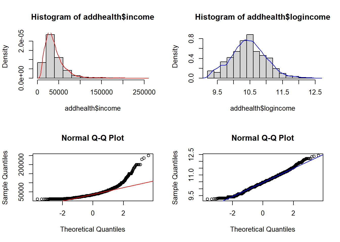
Identify variables
- Quantitative outcome that has been log transformed: Income (variable
logincome) - Binary predictor: Ever smoked a cigarette (variable
eversmoke_c) - Binary confounder: Gender (variable
female_c)
The mathematical multivariable model looks like:
\[ln(Y) \sim \beta_{0} + \beta_{1}x_{1} + \beta_{2}x_{2}\]
Fit a linear regression model
| Estimate | Std. Error | t value | Pr(>|t|) | |
|---|---|---|---|---|
| (Intercept) | 10.65 | 0.026 | 409.8 | 0 |
| wakeup | -0.01491 | 0.003218 | -4.633 | 3.73e-06 |
| female_cFemale | -0.1927 | 0.017 | -11.34 | 2.564e-29 |
| Observations | Residual Std. Error | \(R^2\) | Adjusted \(R^2\) |
|---|---|---|---|
| 3813 | 0.5233 | 0.03611 | 0.0356 |
1-exp(confint(ln.mod.2)[-1,])
##                     2.5 %      97.5 %
## wakeup         0.02099299 0.008561652
## female_cFemale 0.20231394 0.147326777
Interpret the results
- For every hour later one wakes up in the morning, one can expect to earn
1-exp(-0.015)= 1.4% less income than someone who wakes up one hour earlier. This is after controlling for gender. - Females have on average
1-exp(-0.19)= 17% percent lower income than males, after controlling for the wake up time.
Both gender and time one wakes up are significantly associated with the amount of personal earnings one makes. Waking up later in the morning is associated with 1.4% (95% CI 0.8%-2%, p<.0001) percent lower income than someone who wakes up one hour earlier. Females have 17% (95% CI 15%-20%, p<.0001) percent lower income than males.