10.4 Variable Selection Process

Corresponding PMA6 Ch 9

Variable selection methods such as the ones described in this section, are most often used when performing an Exploratory analysis, where many independent variables have been measured, but a final model to explain the variability of a dependent variable has not yet been determined.

When building a model, we want to choose a set of independent variables that both will yield a good prediction using as few variables as possible (parsimony). We also need to consider controlling for moderators and confounders. In many situations where regression is used, the investigator has strong justification for including certain variables in the model.

previous studies
accepted theory

The investigator may have prior justification for using certain variables but may be open to suggestions for the remaining variables.

The set of independent variables can be broken down into logical subsets

Factors of primary interest. (such as an exposure or treatment)
Potential confounders. These are measures that could be associated with both the response, and explanatory variables, and which could explain the relationship between the primary factor of interest and the outcome. These are typically a set of demographics such as age, gender, ethnicity, and tend to be factors found to be important in prior studies.
Effect Modifiers (Moderators). A set of variables that other studies have shown to change or affect the relationship between the explanatory and response variables.
Precision variables (covariates). Variables associated with the dependent variable, but not the primary factor of interest.

How variables are chosen for inclusion into a model is heavily driven by the purpose of the model:

descriptive
predictive

10.4.1 Automated selection procedures (PMA6 9.6)

This example uses the penguins data to model the body mass

The model fitting must apply the models to the same dataset. This may be a problem if there are missing values. We suggest you remove the missing values first. (From the R help file)

pen.nomiss <- pen %>% na.omit()

10.4.1.1 Forward selection: Variables are added one at a time until optimal model reached.

Choose the variable with the highest absolute correlation \(\mid r \mid\) with the outcome.
Choose the next variable that maximizes the model adjusted \(R^{2}\).
Repeat until adding additional variables does not improve the model fit significantly.

10.4.1.2 Backward elimination: Variables are removed one at a time until optimal model reached

Put all variables into the model.
Remove the least useful variable in the model. This can be done by choosing the variable with the largest \(p\)-value.
Repeat until removing additional variables reduces the model fit significantly.

10.4.1.3 Stepwise selection: Combination of forward and backward.

Start with no variables (just \(\bar{Y}\))
Add the variable that results in the greatest improvement in model fit.
Add another variable that results in the greatest improvement in model fit after controlling for the first.
Check to see if removing any variable currently in the model improves the fit.
Add another variable…
Check to remove variables…
Repeat until no variables can be added or removed.

Most programs have the option to force variables to be included in the model. This is important in cases where there is a primary factor of interest such as a treatment effect.

Doing stepwise selection in R

First you need to specify your null model - just the outcome, no covariates, and the full model - the outcome against ALL of your covariates.

null.model <- lm(body_mass_g ~ 1, data=pen.nomiss)
full.model <- lm(body_mass_g ~ ., data=pen.nomiss)

Forward selection

step(null.model, 
     scope=list(lower=null.model, upper=full.model),
     direction='forward', trace=1) |> summary()
## Start:  AIC=4457.28
## body_mass_g ~ 1
## 
##                     Df Sum of Sq       RSS    AIC
## + flipper_length_mm  1 164047703  51211963 3981.1
## + species            2 145190219  70069447 4087.5
## + island             2  83740680 131518986 4297.2
## + bill_length_mm     1  74792533 140467133 4317.1
## + bill_depth_mm      1  47959592 167300074 4375.3
## + sex                1  38878897 176380769 4392.9
## <none>                           215259666 4457.3
## + year               1    102884 215156782 4459.1
## 
## Step:  AIC=3981.13
## body_mass_g ~ flipper_length_mm
## 
##                  Df Sum of Sq      RSS    AIC
## + sex             1   9416589 41795374 3915.5
## + species         2   5368818 45843144 3948.3
## + island          2   3437527 47774435 3962.0
## + year            1   2666295 48545668 3965.3
## + bill_depth_mm   1    338887 50873075 3980.9
## <none>                        51211963 3981.1
## + bill_length_mm  1    140000 51071963 3982.2
## 
## Step:  AIC=3915.47
## body_mass_g ~ flipper_length_mm + sex
## 
##                  Df Sum of Sq      RSS    AIC
## + species         2  13141806 28653568 3793.8
## + island          2   6037165 35758209 3867.5
## + bill_depth_mm   1   3667377 38127997 3886.9
## + year            1   2276715 39518658 3898.8
## <none>                        41795374 3915.5
## + bill_length_mm  1    144990 41650383 3916.3
## 
## Step:  AIC=3793.76
## body_mass_g ~ flipper_length_mm + sex + species
## 
##                  Df Sum of Sq      RSS    AIC
## + bill_depth_mm   1   1196096 27457472 3781.6
## + bill_length_mm  1    780776 27872792 3786.6
## + year            1    474080 28179488 3790.2
## <none>                        28653568 3793.8
## + island          2     61695 28591873 3797.0
## 
## Step:  AIC=3781.56
## body_mass_g ~ flipper_length_mm + sex + species + bill_depth_mm
## 
##                  Df Sum of Sq      RSS    AIC
## + bill_length_mm  1    541825 26915647 3776.9
## + year            1    272828 27184644 3780.2
## <none>                        27457472 3781.6
## + island          2     59488 27397984 3784.8
## 
## Step:  AIC=3776.93
## body_mass_g ~ flipper_length_mm + sex + species + bill_depth_mm + 
##     bill_length_mm
## 
##          Df Sum of Sq      RSS    AIC
## + year    1    319160 26596486 3775.0
## <none>                26915647 3776.9
## + island  2     56214 26859432 3780.2
## 
## Step:  AIC=3774.95
## body_mass_g ~ flipper_length_mm + sex + species + bill_depth_mm + 
##     bill_length_mm + year
## 
##          Df Sum of Sq      RSS  AIC
## <none>                26596486 3775
## + island  2     79468 26517018 3778
## 
## Call:
## lm(formula = body_mass_g ~ flipper_length_mm + sex + species + 
##     bill_depth_mm + bill_length_mm + year, data = pen.nomiss)
## 
## Residuals:
##     Min      1Q  Median      3Q     Max 
## -809.15 -179.43   -3.42  183.60  866.03 
## 
## Coefficients:
##                    Estimate Std. Error t value Pr(>|t|)    
## (Intercept)       80838.770  41677.817   1.940 0.053292 .  
## flipper_length_mm    18.064      3.088   5.849 1.20e-08 ***
## sexmale             382.168     47.797   7.996 2.28e-14 ***
## speciesChinstrap   -274.496     81.558  -3.366 0.000855 ***
## speciesGentoo       929.275    136.036   6.831 4.16e-11 ***
## bill_depth_mm        60.749     19.926   3.049 0.002487 ** 
## bill_length_mm       18.997      7.086   2.681 0.007718 ** 
## year                -41.139     20.832  -1.975 0.049131 *  
## ---
## Signif. codes:  0 '***' 0.001 '**' 0.01 '*' 0.05 '.' 0.1 ' ' 1
## 
## Residual standard error: 286.1 on 325 degrees of freedom
## Multiple R-squared:  0.8764, Adjusted R-squared:  0.8738 
## F-statistic: 329.3 on 7 and 325 DF,  p-value: < 2.2e-16

Backward selection

step(full.model, direction='backward', trace=1) |> summary()
## Start:  AIC=3777.96
## body_mass_g ~ species + island + bill_length_mm + bill_depth_mm + 
##     flipper_length_mm + sex + year
## 
##                     Df Sum of Sq      RSS    AIC
## - island             2     79468 26596486 3775.0
## <none>                           26517018 3778.0
## - year               1    342414 26859432 3780.2
## - bill_length_mm     1    583730 27100748 3783.2
## - bill_depth_mm      1    758473 27275491 3785.3
## - flipper_length_mm  1   2872068 29389086 3810.2
## - sex                1   5101785 31618803 3834.6
## - species            2   6470784 32987802 3846.7
## 
## Step:  AIC=3774.95
## body_mass_g ~ species + bill_length_mm + bill_depth_mm + flipper_length_mm + 
##     sex + year
## 
##                     Df Sum of Sq      RSS    AIC
## <none>                           26596486 3775.0
## - year               1    319160 26915647 3776.9
## - bill_length_mm     1    588158 27184644 3780.2
## - bill_depth_mm      1    760657 27357143 3782.3
## - flipper_length_mm  1   2800047 29396533 3806.3
## - sex                1   5231718 31828204 3832.8
## - species            2   9693667 36290153 3874.4
## 
## Call:
## lm(formula = body_mass_g ~ species + bill_length_mm + bill_depth_mm + 
##     flipper_length_mm + sex + year, data = pen.nomiss)
## 
## Residuals:
##     Min      1Q  Median      3Q     Max 
## -809.15 -179.43   -3.42  183.60  866.03 
## 
## Coefficients:
##                    Estimate Std. Error t value Pr(>|t|)    
## (Intercept)       80838.770  41677.817   1.940 0.053292 .  
## speciesChinstrap   -274.496     81.558  -3.366 0.000855 ***
## speciesGentoo       929.275    136.036   6.831 4.16e-11 ***
## bill_length_mm       18.997      7.086   2.681 0.007718 ** 
## bill_depth_mm        60.749     19.926   3.049 0.002487 ** 
## flipper_length_mm    18.064      3.088   5.849 1.20e-08 ***
## sexmale             382.168     47.797   7.996 2.28e-14 ***
## year                -41.139     20.832  -1.975 0.049131 *  
## ---
## Signif. codes:  0 '***' 0.001 '**' 0.01 '*' 0.05 '.' 0.1 ' ' 1
## 
## Residual standard error: 286.1 on 325 degrees of freedom
## Multiple R-squared:  0.8764, Adjusted R-squared:  0.8738 
## F-statistic: 329.3 on 7 and 325 DF,  p-value: < 2.2e-16

Stepwise

step(null.model, 
     scope=list(lower=null.model, upper=full.model),
     direction='both', trace=1) |> summary()
## Start:  AIC=4457.28
## body_mass_g ~ 1
## 
##                     Df Sum of Sq       RSS    AIC
## + flipper_length_mm  1 164047703  51211963 3981.1
## + species            2 145190219  70069447 4087.5
## + island             2  83740680 131518986 4297.2
## + bill_length_mm     1  74792533 140467133 4317.1
## + bill_depth_mm      1  47959592 167300074 4375.3
## + sex                1  38878897 176380769 4392.9
## <none>                           215259666 4457.3
## + year               1    102884 215156782 4459.1
## 
## Step:  AIC=3981.13
## body_mass_g ~ flipper_length_mm
## 
##                     Df Sum of Sq       RSS    AIC
## + sex                1   9416589  41795374 3915.5
## + species            2   5368818  45843144 3948.3
## + island             2   3437527  47774435 3962.0
## + year               1   2666295  48545668 3965.3
## + bill_depth_mm      1    338887  50873075 3980.9
## <none>                            51211963 3981.1
## + bill_length_mm     1    140000  51071963 3982.2
## - flipper_length_mm  1 164047703 215259666 4457.3
## 
## Step:  AIC=3915.47
## body_mass_g ~ flipper_length_mm + sex
## 
##                     Df Sum of Sq       RSS    AIC
## + species            2  13141806  28653568 3793.8
## + island             2   6037165  35758209 3867.5
## + bill_depth_mm      1   3667377  38127997 3886.9
## + year               1   2276715  39518658 3898.8
## <none>                            41795374 3915.5
## + bill_length_mm     1    144990  41650383 3916.3
## - sex                1   9416589  51211963 3981.1
## - flipper_length_mm  1 134585395 176380769 4392.9
## 
## Step:  AIC=3793.76
## body_mass_g ~ flipper_length_mm + sex + species
## 
##                     Df Sum of Sq      RSS    AIC
## + bill_depth_mm      1   1196096 27457472 3781.6
## + bill_length_mm     1    780776 27872792 3786.6
## + year               1    474080 28179488 3790.2
## <none>                           28653568 3793.8
## + island             2     61695 28591873 3797.0
## - flipper_length_mm  1   4325617 32979185 3838.6
## - species            2  13141806 41795374 3915.5
## - sex                1  17189576 45843144 3948.3
## 
## Step:  AIC=3781.56
## body_mass_g ~ flipper_length_mm + sex + species + bill_depth_mm
## 
##                     Df Sum of Sq      RSS    AIC
## + bill_length_mm     1    541825 26915647 3776.9
## + year               1    272828 27184644 3780.2
## <none>                           27457472 3781.6
## + island             2     59488 27397984 3784.8
## - bill_depth_mm      1   1196096 28653568 3793.8
## - flipper_length_mm  1   3145834 30603306 3815.7
## - sex                1   7932472 35389944 3864.1
## - species            2  10670525 38127997 3886.9
## 
## Step:  AIC=3776.93
## body_mass_g ~ flipper_length_mm + sex + species + bill_depth_mm + 
##     bill_length_mm
## 
##                     Df Sum of Sq      RSS    AIC
## + year               1    319160 26596486 3775.0
## <none>                           26915647 3776.9
## + island             2     56214 26859432 3780.2
## - bill_length_mm     1    541825 27457472 3781.6
## - bill_depth_mm      1    957145 27872792 3786.6
## - flipper_length_mm  1   2481143 29396790 3804.3
## - sex                1   5482024 32397671 3836.7
## - species            2  11183644 38099291 3888.6
## 
## Step:  AIC=3774.95
## body_mass_g ~ flipper_length_mm + sex + species + bill_depth_mm + 
##     bill_length_mm + year
## 
##                     Df Sum of Sq      RSS    AIC
## <none>                           26596486 3775.0
## - year               1    319160 26915647 3776.9
## + island             2     79468 26517018 3778.0
## - bill_length_mm     1    588158 27184644 3780.2
## - bill_depth_mm      1    760657 27357143 3782.3
## - flipper_length_mm  1   2800047 29396533 3806.3
## - sex                1   5231718 31828204 3832.8
## - species            2   9693667 36290153 3874.4
## 
## Call:
## lm(formula = body_mass_g ~ flipper_length_mm + sex + species + 
##     bill_depth_mm + bill_length_mm + year, data = pen.nomiss)
## 
## Residuals:
##     Min      1Q  Median      3Q     Max 
## -809.15 -179.43   -3.42  183.60  866.03 
## 
## Coefficients:
##                    Estimate Std. Error t value Pr(>|t|)    
## (Intercept)       80838.770  41677.817   1.940 0.053292 .  
## flipper_length_mm    18.064      3.088   5.849 1.20e-08 ***
## sexmale             382.168     47.797   7.996 2.28e-14 ***
## speciesChinstrap   -274.496     81.558  -3.366 0.000855 ***
## speciesGentoo       929.275    136.036   6.831 4.16e-11 ***
## bill_depth_mm        60.749     19.926   3.049 0.002487 ** 
## bill_length_mm       18.997      7.086   2.681 0.007718 ** 
## year                -41.139     20.832  -1.975 0.049131 *  
## ---
## Signif. codes:  0 '***' 0.001 '**' 0.01 '*' 0.05 '.' 0.1 ' ' 1
## 
## Residual standard error: 286.1 on 325 degrees of freedom
## Multiple R-squared:  0.8764, Adjusted R-squared:  0.8738 
## F-statistic: 329.3 on 7 and 325 DF,  p-value: < 2.2e-16

Warnings:

Stopping criteria and algorithm can be different for different software programs.
Can reject perfectly plausible models from later consideration
Hides relationships between variables (X3 is added and now X1 is no longer significant. X1 vs X3 should be looked at)

Other references Stats 191 at Stanford. This one uses cross-validation on the stepwise procedures, and demonstrates the dangers of trusting models that come out of blind use of variable selection methods. https://web.stanford.edu/class/stats191/notebooks/Selection.html

10.4.1.4 Best Subsets

Select one X with highest simple \(r\) with Y
Select two X’s with highest multiple \(r\) with Y
Select three X’s with highest multiple \(r\) with Y etc.
Compute adjusted R2, AIC or BIC each time.
Compare and choose among the “best subsets” of various sizes.

oc.ht <- regsubsets(body_mass_g ~ ., data=pen.nomiss)
par(mfrow=c(1,3)) # set plotting window to be 1 row and 3 columns
plot(oc.ht, scale='adjr2');plot(oc.ht, scale='bic');plot(oc.ht, scale='Cp')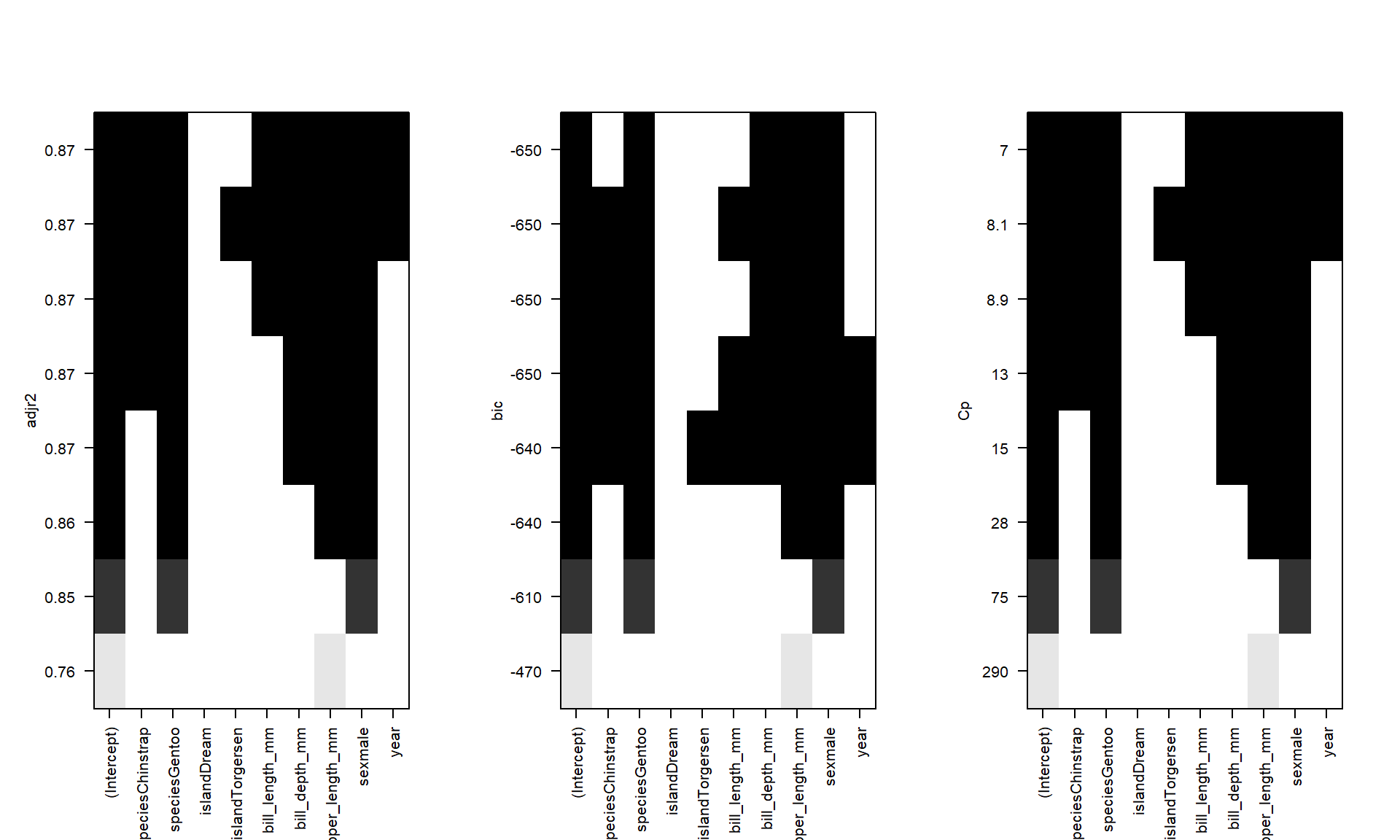

The black squares are when the variable is in the model, the white is when it’s not
The vertical axis are chosen fit metrics such as adjusted R2, BIC and Mallows Cp. The higher the better

In this example variables that show up as improving model fit include species, sex, flipper_length_mm, bill_length, and possibly year. For sure island is out.

Other references from STDHA: http://www.sthda.com/english/articles/37-model-selection-essentials-in-r/155-best-subsets-regression-essentials-in-r/

Notable problems: categorical variables are not treated as a group. that is, they are not “all in” or “all out”. If at least one level is frequently chosen as improving model fit, add the entire categorical variable to the model.

10.4.2 LASSO Regression (PMA6 9.7)

Least Absolute Shrinkage and Selection Operator.

The goal of LASSO is to minimize

\[ RSS + \lambda \sum_{j}\mid \beta_{j} \ \mid \]

where \(\lambda\) is a model complexity penalty parameter.

“Shrinks” the coefficients, setting some to exactly 0.
- Thus essentially choosing a simpler model
Balances model accuracy with interpretation.

The lasso fits many regression models and selects those variables that show the strongest association with the response variable using the data at hand. This is also described as a method of selective inference (Taylor and Tibshirani, 2015) and is an example of exploratory research, where the data may influence what type and how many analyses are performed.

10.4.2.1 Example

This section uses functions glmnet package, and the Chemical data set from PMA6. Also it uses the model.matrix function from the stats package (automatically loaded). This function takes a set of input predictors and turns them into the variables that are used directly in the model. For example, categorical variables will be converted into multiple binary indicators. This typically happens in the background.

The glmnet function works best when the outcome y and predictors x are not contained within a data frame. The alpha argument is the tuning parameter, where a value of 1 specifies the lasso.

library(glmnet)
chem <- read.table("data/Chemical.txt", header = TRUE)
y <- chem$PE
x <- model.matrix(PE~., chem)[,-1] # the -1 drops the intercept
chem.lasso <- glmnet(x, y, alpha = 1)

We can visualize the effect of the coefficient shrinkage using the following plot.

plot(chem.lasso, xvar = "lambda")
mtext(side=3, "Number of Variables", line=2)

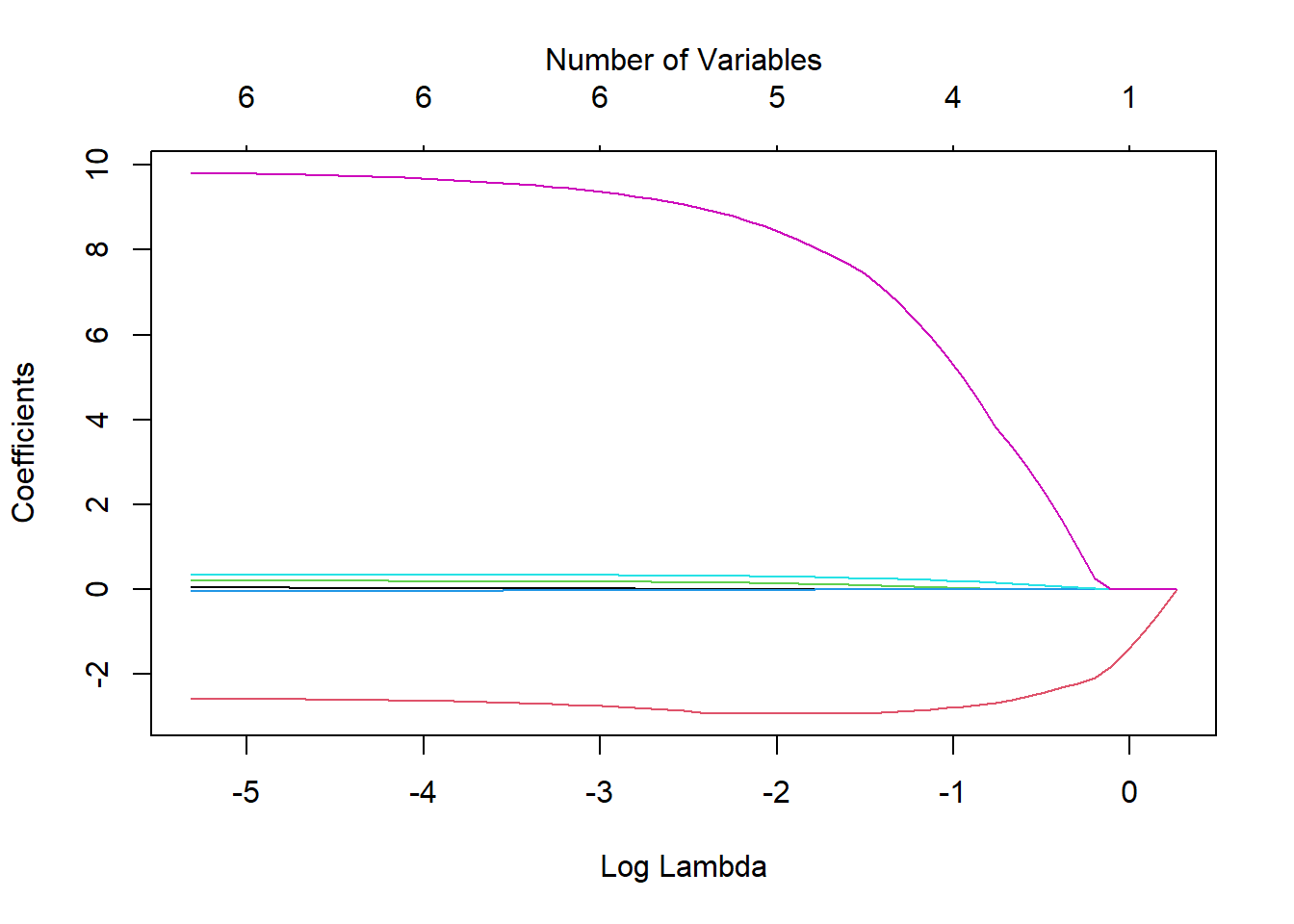
Each line represents the value of a coefficient as \(ln(\lambda)\) changes.
The red line on the bottom and the purple on the top must be important, since they are the last two to be shrunk to 0 and they are relatively stable.

Examining the coefficients of the chem.lasso model object gives us a very large matrix (7x61), listing the coefficients for each value of \(\lambda\) that was tried. A sample of columns are shown below:

coef(chem.lasso)[,1:8]
## 7 x 8 sparse Matrix of class "dgCMatrix"
##                   s0         s1         s2        s3       s4         s5
## (Intercept) 9.366667  9.5835968  9.7812554  9.961355 10.12545 10.0399324
## ROR5        .         .          .          .         .        .        
## DE          .        -0.5206322 -0.9950129 -1.427251 -1.82109 -2.0903355
## SALESGR5    .         .          .          .         .        .        
## EPS5        .         .          .          .         .        .        
## NPM1        .         .          .          .         .        0.0157436
## PAYOUTR1    .         .          .          .         .        0.2427377
##                      s6          s7
## (Intercept)  9.59940208  9.19800729
## ROR5         .           .         
## DE          -2.21050375 -2.31999666
## SALESGR5     .           .         
## EPS5         .           .         
## NPM1         0.04642112  0.07437333
## PAYOUTR1     0.98609790  1.66341998
coef(chem.lasso)[,56:60]
## 7 x 5 sparse Matrix of class "dgCMatrix"
##                     s55         s56         s57         s58         s59
## (Intercept)  1.36957827  1.35834023  1.34802448  1.34099610  1.33052382
## ROR5         0.03767492  0.03797214  0.03825501  0.03840313  0.03870172
## DE          -2.58475249 -2.58199893 -2.57937377 -2.57863116 -2.57530747
## SALESGR5     0.19961031  0.19990639  0.20017553  0.20039468  0.20064382
## EPS5        -0.03468051 -0.03483069 -0.03497088 -0.03507850 -0.03520342
## NPM1         0.34740236  0.34760738  0.34778861  0.34795977  0.34812027
## PAYOUTR1     9.78594052  9.79286717  9.79910767  9.80408094  9.81009965

Comparing the plot to the coefficient model output above, we see that the variables that show up being shrunk last are DE and PAYOUTR1.

Using Cross validation to find minimum lambda

Cross-validation is a resampling method that uses different portions of the data to test and train a model on different iterations Wikipedia.

By applying a cross-validation technique, we can identify the specific value for \(\lambda\) that results in the lowest cross-validated Mean Squared Error (MSE) (\(\lambda_{min}\)). To ensure reproducibility of these results we set a seed for the random number generator prior to analysis.

set.seed(123) # Setting a seed to ensure I get the same results each time I knit
cv.lasso <- cv.glmnet(x, y, alpha = 1) # note change in function

# Fit the final model using the min lambda
model <- glmnet(x, y, alpha = 1, lambda = cv.lasso$lambda.min)

The resulting table of shrunk regression coefficients then is;

coef(model)
## 7 x 1 sparse Matrix of class "dgCMatrix"
##                       s0
## (Intercept)  2.645693621
## ROR5         0.004833458
## DE          -2.882636490
## SALESGR5     0.165581782
## EPS5        -0.017771193
## NPM1         0.323497141
## PAYOUTR1     8.986481946

In this case we would keep variables: DE, SALESGR5, NPM1 and PAYOUTR1. Estimates for ROR5 and EPS56 are very small, and so can be reasonably excluded.

The lasso procedure normalizes the data prior to fitting a model, so the coefficient values that are returned cannot be interpreted directly in context of the problem.
- This does allow us the ability to make “judgement” calls on what is a ‘small’ estimate since it’s no longer dependent on the units of the data.
Appropriate inference after model selection is currently under research. No unifying theory exists yet.
For now, use lasso to choose variables, then fit a model with only those selected variables in the final model.
Variables chosen in this manner are important, yet biased estimates.

lm(PE ~ DE + SALESGR5 + NPM1 + PAYOUTR1, data = chem) |> tbl_regression()

Characteristic	Beta	95% CI¹	p-value
DE	-3.2	-6.9, 0.58	0.094
SALESGR5	0.19	-0.02, 0.41	0.077
NPM1	0.35	0.12, 0.59	0.005
PAYOUTR1	11	4.7, 17	0.001
¹ CI = Confidence Interval

10.4.2.2 Ridge Regression (PMA6 10.6)

Often compared to LASSO, Ridge regression also minimizes the RSS, but the penalty function is different: \[ RSS + \lambda \sum_{j} \beta_{j}^2 \]

Ridge regression only shrinks the magnitude of the coefficients, not set them exactly to zero.

This means Ridge regression is not a method of variable selection.