15.4 Factor Extraction Methods
Methods
- Principal Components
- Iterated Components
- Maximum Likelihood
15.4.1 Principal components (PC Factor model)
Recall that \(\mathbf{C} = \mathbf{A}\mathbf{X}\), C’s are a function of X
\[ C_{1} = a_{11}X_{1} + a_{12}X_{2} + \ldots + a_{1P}X_{p} \]
We want the reverse: X’s are a function of F’s.
- Use the inverse! –> If \(c = 5x\) then \(x = 5^{-1}C\)
The inverse PC model is \(\mathbf{X} = \mathbf{A}^{-1}\mathbf{C}\).
Since \(\mathbf{A}\) is orthogonal, \(\mathbf{A}^{-1} = \mathbf{A}^{T} = \mathbf{A}^{'}\), so
\[ X_{1} = a_{11}C_{1} + a_{21}C_{2} + \ldots + a_{P1}C_{p} \]
But there are more PC’s than Factors…
\[ \begin{equation} \begin{aligned} X_{i} &= \sum_{j=1}^{P}a_{ji}C_{j} \\ &= \sum_{j=1}^{m}a_{ji}C_{j} + \sum_{j=m+1}^{m}a_{ji}C_{j} \\ &= \sum_{j=1}^{m}l_{ji}F_{j} + e_{i} \\ \end{aligned} \end{equation} \]
Adjustment
- \(V(C_{j}) = \lambda_{j}\) not 1
- We transform: \(F_{j} = C_{j}\lambda_{j}^{-1/2}\)
- Now \(V(F_{j}) = 1\)
- Loadings: \(l_{ij} = \lambda_{j}^{1/2}a_{ji}\)
This is similar to \(a_{ij}\) in PCA.
15.4.1.1 R code
Factor extraction via principal components can be done using the principal function in the psych package. We choose nfactors=2 here because we know there are 2 underlying factors in the data generation model.
#library(psych)
pc.extract.norotate <- principal(stan.dta, nfactors=2, rotate="none")
print(pc.extract.norotate)
## Principal Components Analysis
## Call: principal(r = stan.dta, nfactors = 2, rotate = "none")
## Standardized loadings (pattern matrix) based upon correlation matrix
##     PC1   PC2   h2    u2 com
## X1 0.57  0.75 0.89 0.112 1.9
## X2 0.61  0.72 0.89 0.113 1.9
## X3 0.58 -0.51 0.59 0.406 2.0
## X4 0.87 -0.38 0.89 0.109 1.4
## X5 0.92 -0.27 0.91 0.086 1.2
##
##                        PC1  PC2
## SS loadings           2.63 1.55
## Proportion Var        0.53 0.31
## Cumulative Var        0.53 0.83
## Proportion Explained  0.63 0.37
## Cumulative Proportion 0.63 1.00
##
## Mean item complexity =  1.7
## Test of the hypothesis that 2 components are sufficient.
##
## The root mean square of the residuals (RMSR) is  0.09
##  with the empirical chi square  16.62  with prob <  4.6e-05
##
## Fit based upon off diagonal values = 0.96
\[ \begin{equation} \begin{aligned} X_{1} &= 0.53F_{1} + 0.78F_{2} + e_{1} \\ X_{2} &= 0.59F_{1} + 0.74F_{2} + e_{2} \\ X_{3} &= 0.70F_{1} - 0.39F_{2} + e_{3} \\ X_{4} &= 0.87F_{1} - 0.38F_{2} + e_{4} \\ X_{5} &= 0.92F_{1} - 0.27F_{2} + e_{5} \\ \end{aligned} \end{equation} \]
These equations come from the top of the output, under Standardized loadings.
15.4.2 Iterated components
Select common factors to maximize the total communality
- Get initial communality estimates
- Use these (instead of original variances) to get the PC’s and factor loadings
- Get new communality estimates
- Rinse and repeat
- Stop when no appreciable changes occur.
R code not shown, but can be obtained using the factanal package in R.
15.4.3 Maximum Likelihood
- Assume that all the variables are normally distributed
- Use Maximum Likelihood to estimate the parameters
15.4.3.1 R code
The cutoff argument hides loadings under that value for ease of interpretation. Here I am setting that cutoff at 0 so that all loadings are being displayed. I encourage you to adjust this cutoff value in practice to see how it can be useful in reducing cognitave load of looking through a grid of numbers.
ml.extract.norotate <- factanal(stan.dta, factors=2, rotation="none")
print(ml.extract.norotate, digits=2, cutoff=0)
##
## Call:
## factanal(x = stan.dta, factors = 2, rotation = "none")
##
## Uniquenesses:
##   X1   X2   X3   X4   X5
## 0.33 0.06 0.72 0.08 0.01
##
## Loadings:
##    Factor1 Factor2
## X1  0.35    0.74
## X2  0.41    0.88
## X3  0.50   -0.18
## X4  0.94   -0.19
## X5  0.99   -0.07
##
##                Factor1 Factor2
## SS loadings       2.41    1.39
## Proportion Var    0.48    0.28
## Cumulative Var    0.48    0.76
##
## Test of the hypothesis that 2 factors are sufficient.
## The chi square statistic is 0.4 on 1 degree of freedom.
## The p-value is 0.526
The factor equations now are:
\[ \begin{equation} \begin{aligned} X_{1} &= -0.06F_{1} + 0.79F_{2} + e_{1} \\ X_{2} &= -0.07F_{1} + 1F_{2} + e_{2} \\ X_{3} &= 0.58F_{1} + 0.19F_{2} + e_{3} \\ \vdots \end{aligned} \end{equation} \]
15.4.4 Uniqueness
Recall Factor analysis splits the variance of the observed X’s into a part due to the communality \(h_{i}^{2}\) and specificity \(u_{i}^{2}\). This last term is the portion of the variance that is due to the unique factor. Let’s look at how those differ depending on the extraction method:
pc.extract.norotate$uniquenesses
##         X1         X2         X3         X4         X5
## 0.11151283 0.11336123 0.40564130 0.10890203 0.08591098
ml.extract.norotate$uniquenesses
##         X1         X2         X3         X4         X5
## 0.33432315 0.05506386 0.71685548 0.07508356 0.01414656
Here we see that the uniqueness for X2, X4 and X5 under ML is pretty low compared to the PC extraction method, but that’s almost offset by a much higher uniqueness for x1 and X3.
Ideally we want the variance in the X’s to be captured by the factors. So we want to see a low unique variance.
15.4.5 Resulting factors
par(mfrow=c(1,2)) # grid of 2 columns and 1 row

pc.load <- pc.extract.norotate$loadings[,1:2]
plot(pc.load, type="n", main="PCA Extraction") # set up the plot but don't put points down
text(pc.load, labels=rownames(pc.load)) # put names instead of points

ml.load <- ml.extract.norotate$loadings[,1:2]
plot(ml.load, type="n", main="ML Extraction")
text(ml.load, labels=rownames(ml.load))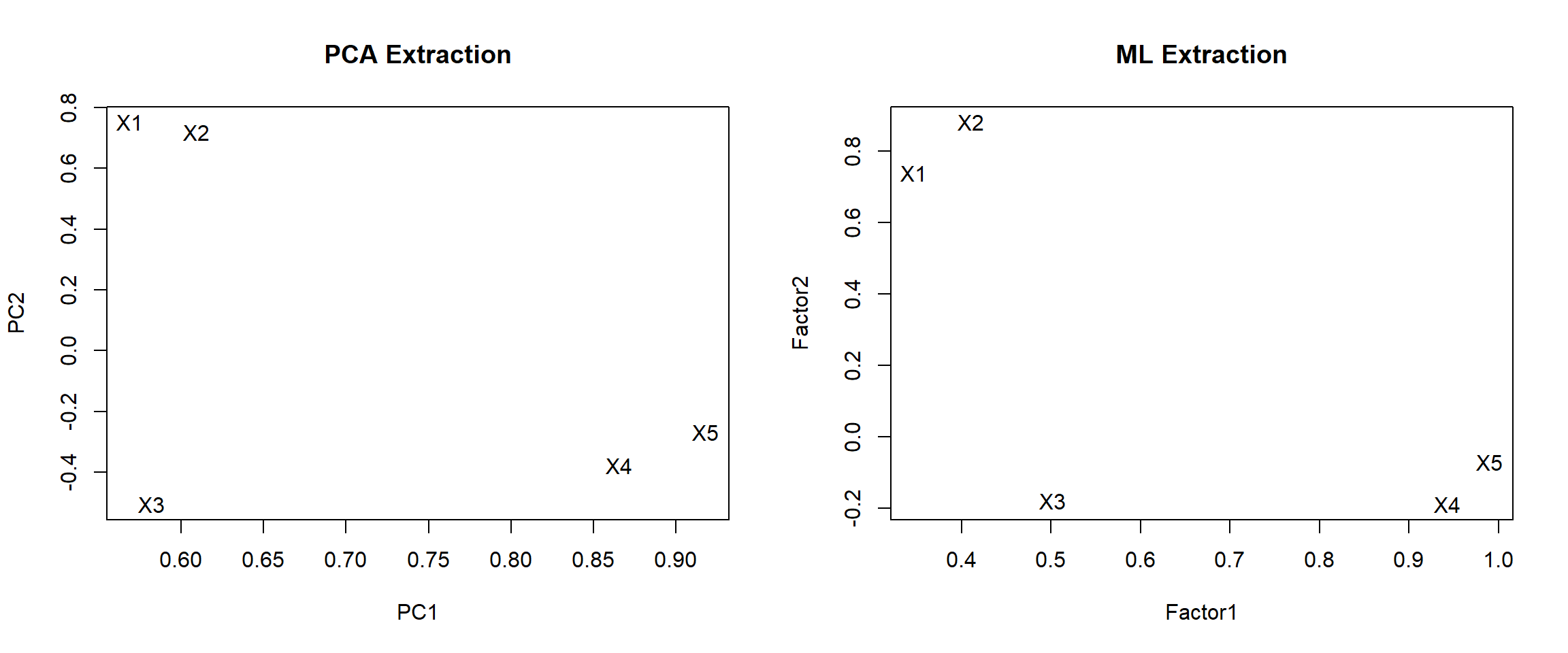
PCA Extraction
- X1 and X2 load high on PC1, and low on PC1.
- X3, 4 and 5 are negative on PC2, and moderate to high on PC1.
- PC1 is not highly correlated with X3
ML Extraction
- Same overall split, X3 still not loading high on Factor 1.
- X1 loading lower on Factor 2 compared to PCA extraction method.
Neither extraction method reproduced our true hypothetical factor model. Rotating the factors will achieve our desired results.