18.9 Example: Prescribed amount of missing.
We will demonstrate using the Palmer Penguins dataset where we can artificially create a prespecified percent of the data missing, (after dropping the 11 rows missing sex) This allows us to be able to estimate the bias incurred by using these imputation methods.
For the penguin data ) out we set a seed and use the prodNA() function from the missForest package to create 10% missing values in this data set.
library(missForest)
set.seed(12345) # Raspberry, I HATE raspberry!
pen.nomiss <- na.omit(pen)
pen.miss <- prodNA(pen.nomiss, noNA=0.1)
prop.table(table(is.na(pen.miss)))
##
##      FALSE       TRUE
## 0.90015015 0.09984985
Visualize missing data pattern.
aggr(pen.miss, col=c('darkolivegreen3','salmon'),
              numbers=TRUE, sortVars=TRUE,
              labels=names(pen.miss), cex.axis=.7,
              gap=3, ylab=c("Missing data","Pattern"))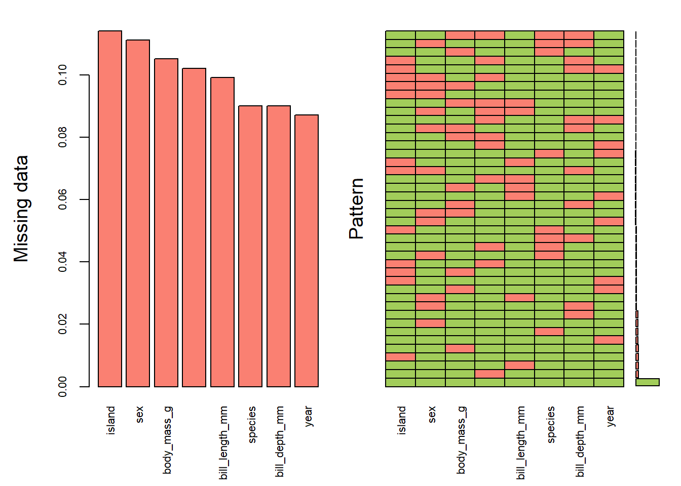
##
##  Variables sorted by number of missings:
##           Variable      Count
##             island 0.11411411
##                sex 0.11111111
##        body_mass_g 0.10510511
##  flipper_length_mm 0.10210210
##     bill_length_mm 0.09909910
##            species 0.09009009
##      bill_depth_mm 0.09009009
##               year 0.08708709
Here’s another example of where only 10% of the data overall is missing, but it results in only 58% complete cases.
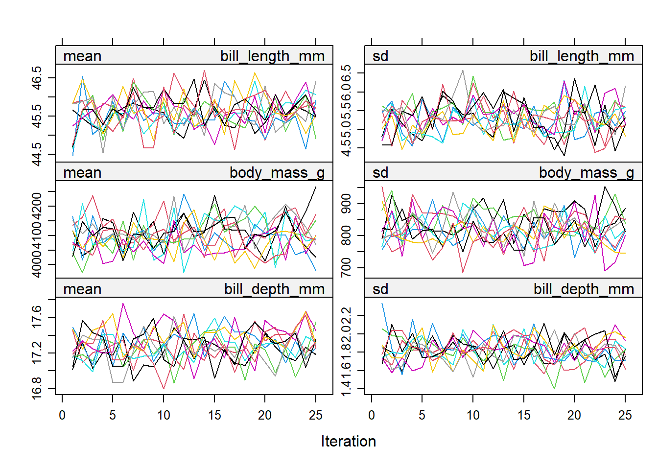
18.9.1 Multiply impute the missing data using mice()
imp_pen <- mice(pen.miss, m=10, maxit=25, meth="pmm", seed=500, printFlag=FALSE)
summary(imp_pen)
## Class: mids
## Number of multiple imputations:  10
## Imputation methods:
##           species            island    bill_length_mm     bill_depth_mm
##             "pmm"             "pmm"             "pmm"             "pmm"
## flipper_length_mm       body_mass_g               sex              year
##             "pmm"             "pmm"             "pmm"             "pmm"
## PredictorMatrix:
##                   species island bill_length_mm bill_depth_mm flipper_length_mm
## species                 0      1              1             1                 1
## island                  1      0              1             1                 1
## bill_length_mm          1      1              0             1                 1
## bill_depth_mm           1      1              1             0                 1
## flipper_length_mm       1      1              1             1                 0
## body_mass_g             1      1              1             1                 1
##                   body_mass_g sex year
## species                     1   1    1
## island                      1   1    1
## bill_length_mm              1   1    1
## bill_depth_mm               1   1    1
## flipper_length_mm           1   1    1
## body_mass_g                 0   1    1
The Stack Exchange post listed below has a great explanation/description of what each of these arguments control. It is a very good idea to understand these controls.
https://stats.stackexchange.com/questions/219013/how-do-the-number-of-imputations-the-maximum-iterations-affect-accuracy-in-mul/219049#21904918.9.2 Check the imputation method used on each variable.
imp_pen$meth
##           species            island    bill_length_mm     bill_depth_mm
##             "pmm"             "pmm"             "pmm"             "pmm"
## flipper_length_mm       body_mass_g               sex              year
##             "pmm"             "pmm"             "pmm"             "pmm"
Predictive mean matching was used for all variables, even species and island. This is reasonable because PMM is a hot deck method of imputation.
18.9.4 Look at the values generated for imputation
imp_pen$imp$body_mass_g |> head()
##       1    2    3    4    5    6    7    8    9   10
## 3  3800 3750 3550 3900 3550 3300 3400 3900 3450 3900
## 8  3300 3150 3525 3150 3500 3150 3325 3200 3325 3300
## 13 4300 4050 4500 4000 4675 4550 4050 3950 4575 4550
## 35 3400 3900 4075 3600 3900 3700 3900 3425 4725 3250
## 41 3600 4300 3900 3600 3950 3900 3500 3900 4150 4100
## 45 2700 3100 3625 3700 3525 3800 3575 3100 3575 3525
This is just for us to see what this imputed data look like. Each column is an imputed value, each row is a row where an imputation for body_mass_g was needed. Notice only imputations are shown, no observed data is showing here.
18.9.5 Create a complete data set by filling in the missing data using the imputations
Action=1 returns the first completed data set, action=2 returns the second completed data set, and so on.
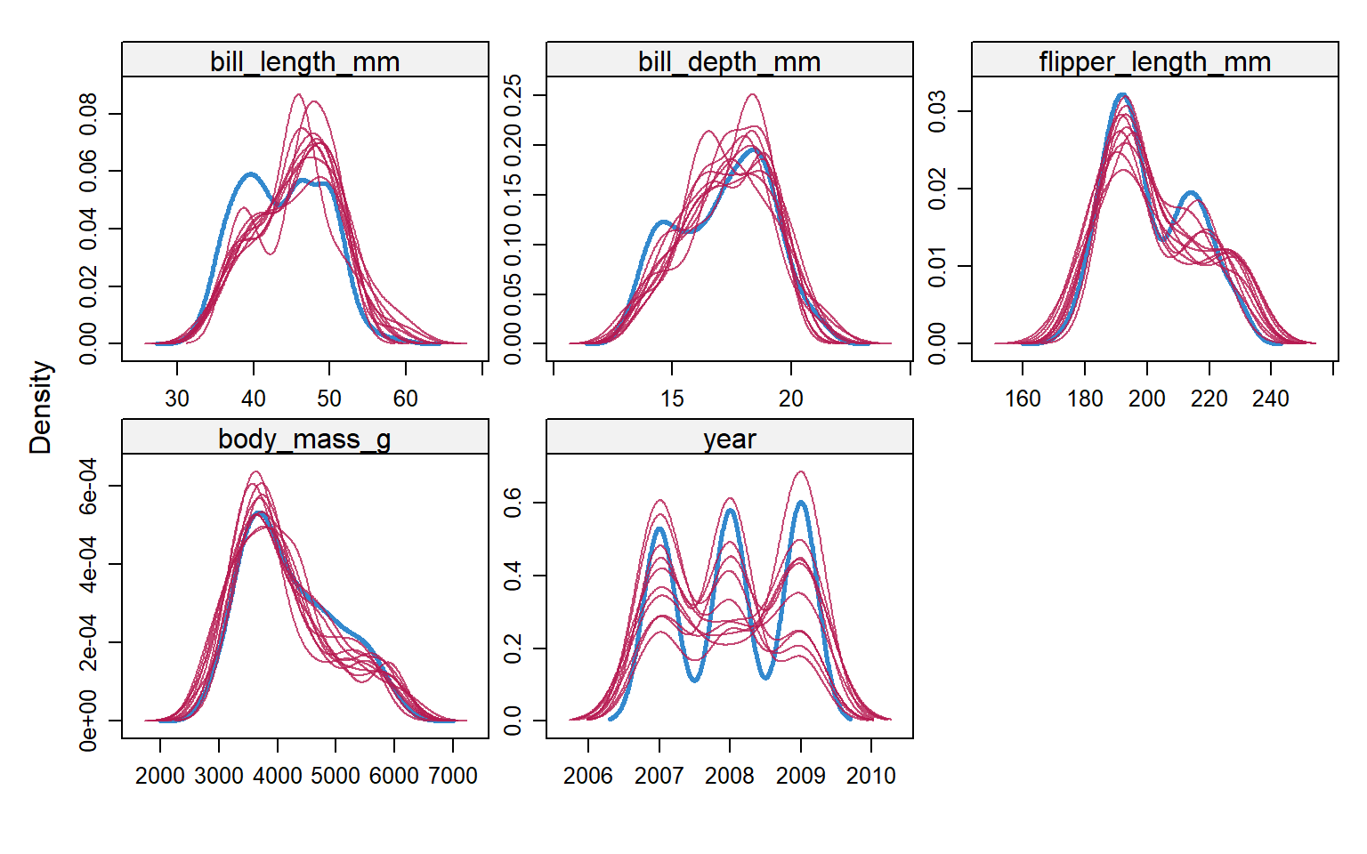
18.9.6 Visualize Imputations
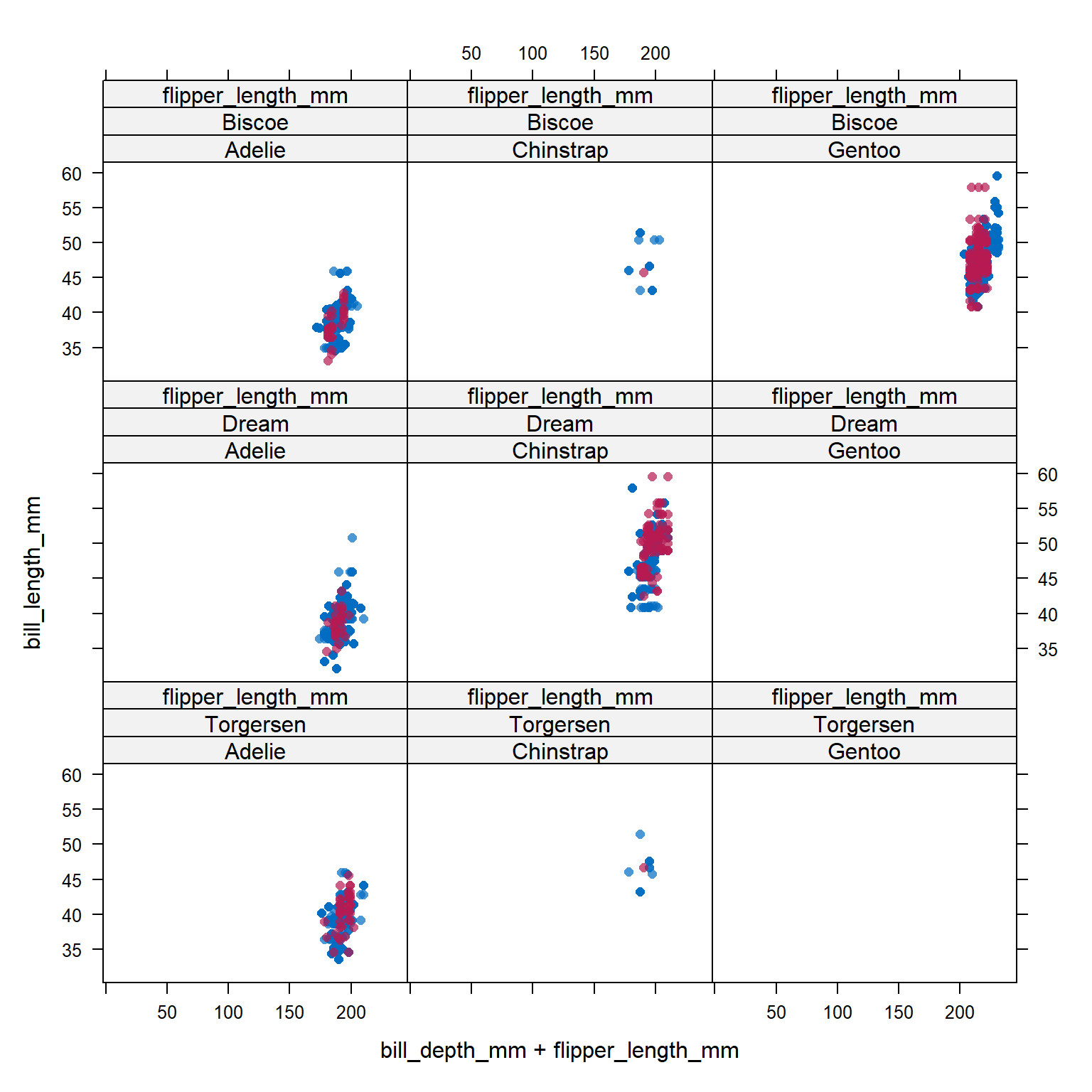
Let’s compare the imputed values to the observed values to see if they are indeed “plausible” We want to see that the distribution of of the magenta points (imputed) matches the distribution of the blue ones (observed).
Univariately
Multivariately
xyplot(imp_pen, bill_length_mm ~ bill_depth_mm + flipper_length_mm | species + island, cex=.8, pch=16)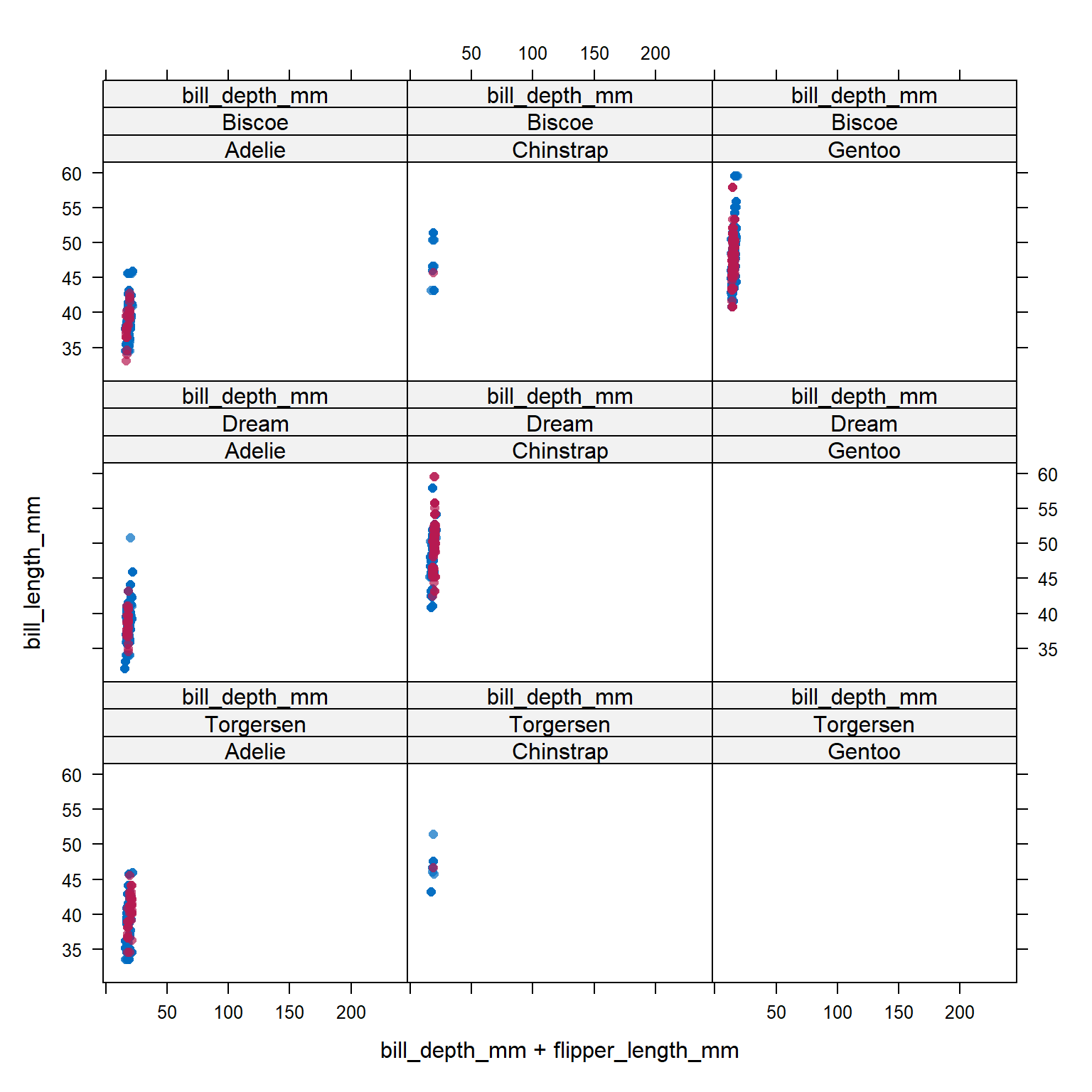
Analyze and pool All of this imputation was done so we could actually perform an analysis!
Let’s run a simple linear regression on body_mass_g as a function of bill_length_mm, flipper_length_mm and species.
model <- with(imp_pen, lm(body_mass_g ~ bill_length_mm + flipper_length_mm + species))
summary(pool(model))
##                term    estimate  std.error statistic        df      p.value
## 1       (Intercept) -3758.87511 577.502100 -6.508851 205.80708 5.670334e-10
## 2    bill_length_mm    51.61565   9.013278  5.726624  49.20373 6.081152e-07
## 3 flipper_length_mm    28.67977   3.819019  7.509722  84.41687 5.618897e-11
## 4  speciesChinstrap  -615.76862  97.112862 -6.340753  68.84331 2.051941e-08
## 5     speciesGentoo   155.61083  92.618867  1.680120 298.97391 9.397845e-02
Pooled parameter estimates \(\bar{Q}\) and their standard errors \(\sqrt{T}\) are provided, along with a significance test (against \(\beta_p=0\)). Note with this output that a 95% interval must be calculated manually.
We can leverage the gtsummary package to tidy and print the results of a mids object, but the mice object has to be passed to tbl_regression BEFORE you pool. ref SO post. This function needs to access features of the original model first, then will do the appropriate pooling and tidying.
| Characteristic | Beta | 95% CI1 | p-value |
|---|---|---|---|
| bill_length_mm | 52 | 34, 70 | <0.001 |
| flipper_length_mm | 29 | 21, 36 | <0.001 |
| species | |||
| Adelie | — | — | |
| Chinstrap | -616 | -810, -422 | <0.001 |
| Gentoo | 156 | -27, 338 | 0.094 |
| 1 CI = Confidence Interval | |||
Additionally digging deeper into the object created by pool(model), specifically the pooled list, we can pull out additional information including the number of missing values, the fraction of missing information (fmi) as defined by Rubin (1987), and lambda, the proportion of total variance that is attributable to the missing data (\(\lambda = (B + B/m)/T)\).
| term | m | estimate | ubar | df | riv |
|---|---|---|---|---|---|
| (Intercept) | 10 | -3758.875 | 296028.896 | 205.807 | 0.127 |
| bill_length_mm | 10 | 51.616 | 50.961 | 49.204 | 0.594 |
| flipper_length_mm | 10 | 28.680 | 10.749 | 84.417 | 0.357 |
| speciesChinstrap | 10 | -615.769 | 6583.091 | 68.843 | 0.433 |
| speciesGentoo | 10 | 155.611 | 8255.317 | 298.974 | 0.039 |
18.9.7 Calculating bias
The penguins data set used here had no missing data to begin with. So we can calculate the “true” parameter estimates…
and find the difference in coefficients.
The variance of the multiply imputed estimates is larger because of the between-imputation variance.
tm.est <- true.model |> coef() |> broom::tidy() |> mutate(model = "True Model") |>
  rename(est = x)
tm.est$cil <- confint(true.model)[,1]
tm.est$ciu <- confint(true.model)[,2]
tm.est <- tm.est[-1,] # drop intercept

mi <- tbl_regression(model)$table_body |>
  select(names = label, est = estimate, cil=conf.low, ciu=conf.high) |>
  mutate(model = "MI") |> filter(!is.na(est))

pen.mi.compare <- bind_rows(tm.est, mi)
pen.mi.compare$names <- gsub("species", "", pen.mi.compare$names)

ggplot(pen.mi.compare, aes(x=est, y = names, col=model)) +
  geom_point() + geom_errorbar(aes(xmin=cil, xmax=ciu), width=0.2) +
theme_bw() 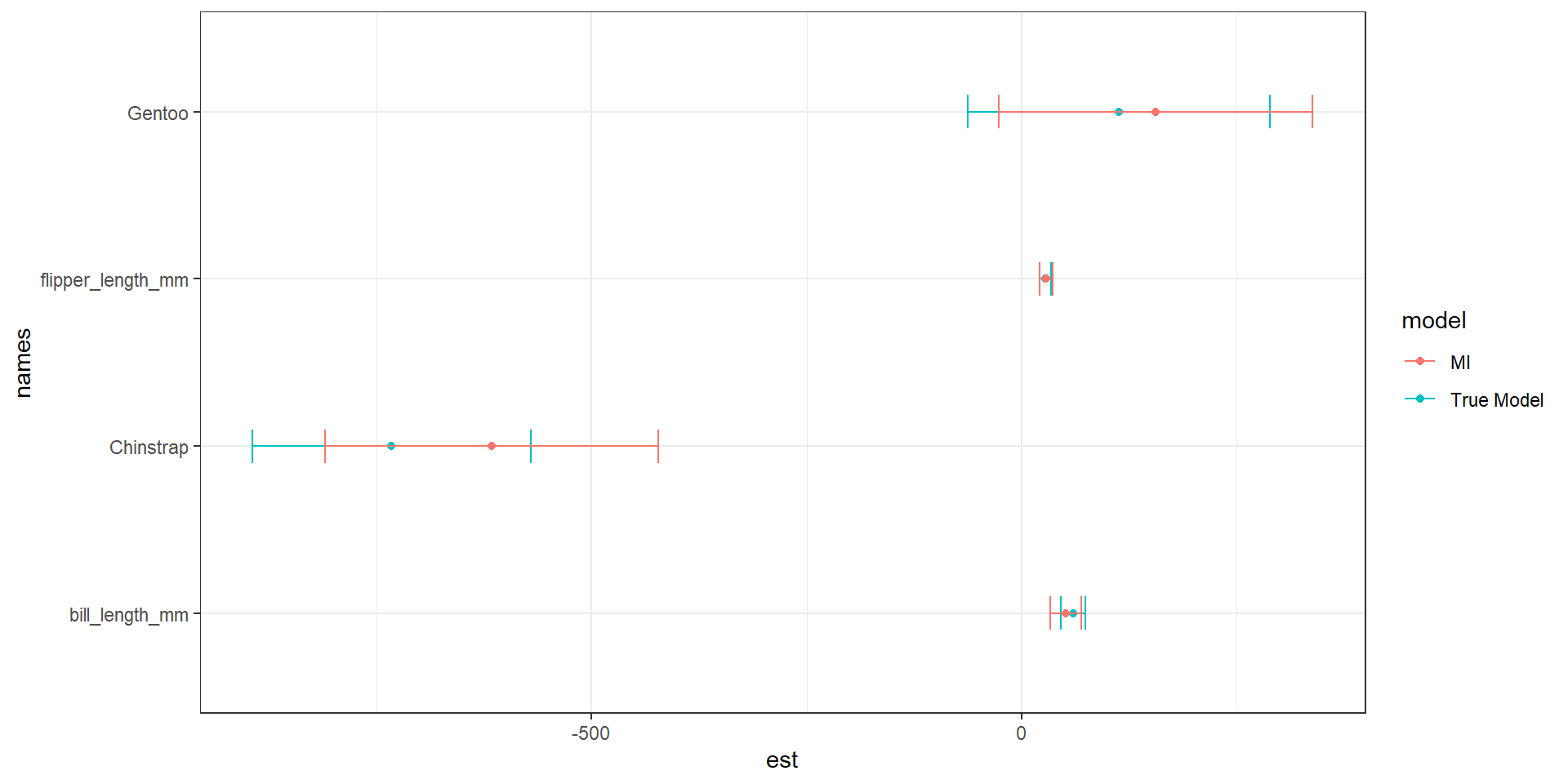
| names | True Model | MI | bias |
|---|---|---|---|
| bill_length_mm | 60.11732 | 51.61565 | -8.501672 |
| flipper_length_mm | 27.54429 | 28.67977 | 1.135481 |
| Chinstrap | -732.41667 | -615.76862 | 116.648049 |
| Gentoo | 113.25418 | 155.61083 | 42.356655 |
MI over estimates the difference in body mass between Chinstrap and Adelie, but underestiamtes that difference for Gentoo. There is also an underestimation of the relationship between bill length and body mass.