18.3 Missing Data Mechanisms

Process by which some units observed, some units not observed

Missing Completely at Random (MCAR): The probability that a data point is missing is completely unrelated (independent) of any observed and unobserved data or parameters.
- P(Y missing| X, Y) = P(Y missing)
- Ex: Miscoding or forgetting to log in answer
Missing at Random (MAR): The probability that a data point is missing is independent can be explained or modeled by other observed variables.
- P(Y missing|x, Y) = P(Y missing | X)
- Ex: Y = age, X = sex
  - Pr (Y miss| X = male) = 0.2
  - Pr (Y miss| X = female) = 0.3
  - Males people are less likely to fill out an income survey - The missing data on income is related to gender - After accounting for gender the missing data is unrelated to income.
Not missing at Random (NMAR): The probability that a data point is missing depends on the value of the variable in question.
- P(Y missing | X, Y) = P (Y missing|X, Y)
- Ex: Y = income, X = immigration status
  - Richer person may be less willing to disclose income
  - Undocumented immigrant may be less willing to disclose income

Write down an example of each.

Does it matter to inferences? Yes!

18.3.1 Demonstration via Simulation

What follows is just one method of approaching this problem via code. Simulation is a frequently used technique to understand the behavior of a process over time or over repeated samples.

18.3.1.1 MCAR

Draw a random sample of size 100 from a standard Normal distribution (Z) and calculate the mean.

set.seed(456) # setting a seed ensures the same numbers will be drawn each time
z <- rnorm(100)
mean.z <- mean(z)
mean.z
## [1] 0.1205748

Delete data at a rate of $p$ and calculate the complete case (available) mean.
- Sample 100 random Bernoulli (0/1) variables with probability $p$.
```
x <- rbinom(100, 1, p=.5)
```
- Find out which elements are are 1’s
```
delete.these <- which(x==1)
```
- Set those elements in z to NA.
```
z[delete.these] <- NA
```
- Calculate the complete case mean
```
mean(z, na.rm=TRUE)
## [1] 0.1377305
```
Calculate the bias as the sample mean minus the true mean ($E(\hat\theta) - \theta$).

mean(z, na.rm=TRUE) - mean.z
## [1] 0.01715565

How does the bias change as a function of the proportion of missing? Let $p$ range from 0% to 99% and plot the bias as a function of $p$.

calc.bias <- function(p){ # create a function to handle the repeated calculations
  mean(ifelse(rbinom(100, 1, p)==1, NA, z), na.rm=TRUE) - mean.z
}

p <- seq(0,.99,by=.01)

plot(c(0,1), c(-1, 1), type="n", ylab="Bias", xlab="Proportion of missing")
  points(p, sapply(p, calc.bias), pch=16)
  abline(h=0, lty=2, col="blue")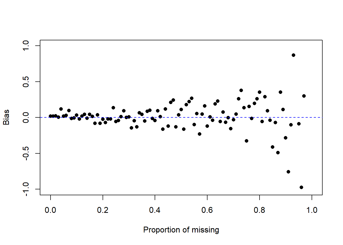

What is the behavior of the bias as $p$ increases? Look specifically at the position/location of the bias, and the variance/variability of the bias.

18.3.1.2 NMAR: Missing related to data

What if the rate of missing is related to the value of the outcome? Again, let’s setup a simulation to see how this works.

Randomly draw 100 random data points from a Standard Normal distribution to serve as our population, and 100 uniform random values between 0 and 1 to serve as probabilities of the data being missing ($p=P(miss)$)

Z <- rnorm(100)
p <- runif(100, 0, 1)

Sort both in ascending order, shove into a data frame and confirm that $p(miss)$ increases along with $z$.

dta <- data.frame(Z=sort(Z), p=sort(p))
head(dta)
##           Z           p
## 1 -2.898122 0.003673455
## 2 -2.185058 0.013886146
## 3 -2.076032 0.035447986
## 4 -1.938288 0.039780643
## 5 -1.930809 0.051362816
## 6 -1.905331 0.054639596
ggplot(dta, aes(x=p, y=Z)) + geom_point() + xlab("P(missing)") + ylab("Z~Normal(0,1)")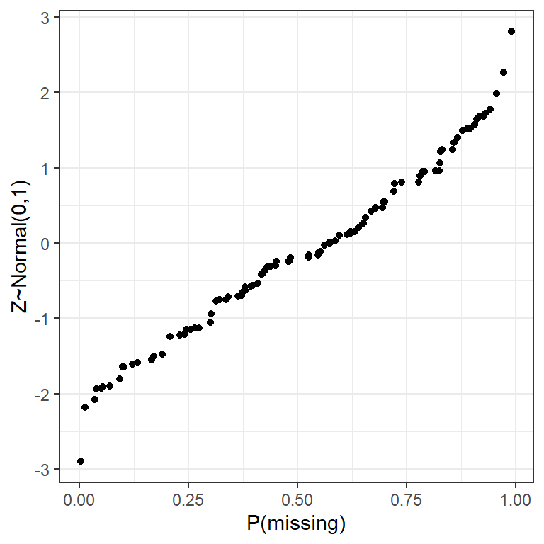

Set $Z$ missing with probability equal to the $p$ for that row. Create a new vector dta$z.miss that is either 0, or the value of dta$Z with probability 1-dta$p. Then change all the 0’s to NA.

dta$Z.miss <- dta$Z * (1-rbinom(NROW(dta), 1, dta$p))
head(dta) # see structure of data to understand what is going on
##           Z           p    Z.miss
## 1 -2.898122 0.003673455 -2.898122
## 2 -2.185058 0.013886146 -2.185058
## 3 -2.076032 0.035447986 -2.076032
## 4 -1.938288 0.039780643 -1.938288
## 5 -1.930809 0.051362816 -1.930809
## 6 -1.905331 0.054639596 -1.905331
dta$Z.miss[dta$Z.miss==0] <- NA

Calculate the complete case mean and the bias

mean(dta$Z.miss, na.rm=TRUE)
## [1] -0.7777319
mean(dta$Z) - mean(dta$Z.miss, na.rm=TRUE)
## [1] 0.6830372

Did the complete case estimate over- or under-estimate the true mean? Is the bias positive or negative?

18.3.1.3 NMAR: Pure Censoring

Consider a hypothetical blood test to measure a hormone that is normally distributed in the blood with mean 10$\mu g$ and variance 1. However the test to detect the compound only can detect levels above 10.

z <- rnorm(100, 10, 1)
y <- z
y[y<10] <- NA
mean(z) - mean(y, na.rm=TRUE)
## [1] -0.6850601

Did the complete case estimate over- or under-estimate the true mean?

When the data is not missing at random, the bias can be much greater.

Usually you don’t know the missing data mechanism.

Degrees of difficulty

MCAR: is easiest to deal with.
MAR: we can live with it.
NMAR: most difficult to handle.

Evidence?

What can we learn from evidence in the data set at hand?

May be evidence in the data rule out MCAR - test responders vs. nonresponders.
- Example: Responders tend to have higher/lower average education than nonresponders by t-test
- Example: Response more likely in one geographic area than another by chi-square test
No evidence in data set to rule out MAR (although there may be evidence from an external data source)

What is plausible?

Cochran example: when human behavior is involved, MCAR must be viewed as an extremely special case that would often be violated in practice
Missing data may be introduced by design (e.g., measure some variables, don’t measure others for reasons of cost, response burden), in which case MCAR would apply
MAR is much more common than MCAR
We cannot be too cavalier about assuming MAR, but anecdotal evidence shows that it often is plausible when conditioning on enough information

Ignorable Missing

If missing-data mechanism is MCAR or MAR then nonresponse is said to be “ignorable”.
Origin of name: in likelihood-based inference, both the data model and missing-data mechanism are important but with MCAR or MAR, inference can be based solely on the data model, thus making inference much simpler
“Ignorability” is a relative assumption: missingness on income may be NMAR given only gender, but may be MAR given gender, age, occupation, region of the country