14.2 Basic Idea - change of coordinates

Consider a hypothetical data set that consists of 100 random pairs of observations \(X_{1}\) and \(X_{2}\) that are correlated. Let \(X_{1} \sim \mathcal{N}(100, 100)\), \(X_{2} \sim \mathcal{N}(50, 50)\), with \(\rho_{12} = \frac{1}{\sqrt{2}}\).

In matrix notation this is written as: \(\mathbf{X} \sim \mathcal{N}\left(\mathbf{\mu}, \mathbf{\Sigma}\right)\) where \[\mathbf{\mu} = \left(\begin{array} {r} \mu_{1} \\ \mu_{2} \end{array}\right), \mathbf{\Sigma} = \left(\begin{array} {cc} \sigma_{1}^{2} & \rho_{12}\sigma_{x}\sigma_{y} \\ \rho_{12}\sigma_{x}\sigma_{y} & \sigma_{2}^{2} \end{array}\right) \].

set.seed(456)
m <- c(100, 50)
s <- matrix(c(100, sqrt(.5*100*50), sqrt(.5*100*50), 50), nrow=2)
data <- data.frame(MASS::mvrnorm(n=100, mu=m, Sigma=s))
colnames(data) <- c("X1", "X2")

plot(X2 ~ X1, data=data, pch=16)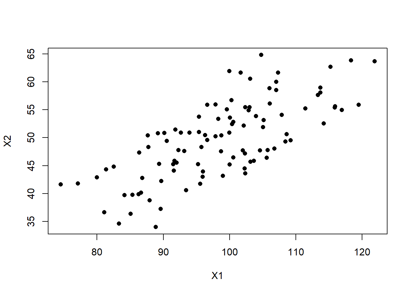

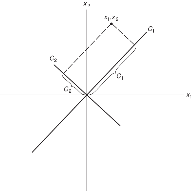
Goal: Create two new variables \(C_{1}\) and \(C_{2}\) as linear combinations of \(\mathbf{x_{1}}\) and \(\mathbf{x_{2}}\)

\[ \mathbf{C_{1}} = a_{11}\mathbf{x_{1}} + a_{12}\mathbf{x_{2}} \] \[ \mathbf{C_{2}} = a_{21}\mathbf{x_{1}} + a_{22}\mathbf{x_{2}} \]

or more simply \(\mathbf{C = aX}\), where

• The \(\mathbf{x}\)’s have been centered by subtracting their mean (\(\mathbf{x_{1}} = x_{1}-\bar{x_{1}}\))
• \(Var(C_{1})\) is as large as possible

Graphically we’re creating two new axes, where now \(C_{1}\) and \(C_{2}\) are uncorrelated.

PCA is mathematically defined as an orthogonal linear transformation that transforms the data to a new coordinate system such that the greatest variance by some projection of the data comes to lie on the first coordinate (called the first principal component), the second greatest variance on the second coordinate, and so on. Wikipedia

In Linear Algebra terms, this is a change of basis. We are changing from a coordinate system of \((x_{1},x_{2})\) to \((c_{1}, c_{2})\). If you want to see more about this concept, here is a good [YouTube Video].