10.6 Model Diagnostics
Recall from Section 7.2 the assumptions for linear regression model are;
- Linearity The relationship between \(x_j\) and \(y\) is linear, for all \(j\).
- Normality, Homogeneity of variance The residuals are identically distributed \(\epsilon_{i} \sim N(0, \sigma^{2})\)
- Uncorrelated/Independent Distinct error terms are uncorrelated: \(\text{Cov}(\epsilon_{i},\epsilon_{j})=0,\forall i\neq j.\)
There are a few ways to visually assess these assumptions. We’ll look at this using a penguin model of body mass as an example.
10.6.1 Linearity
Create a scatterplot with lowess AND linear regression line. See how close the lowess trend line is to the best fit line. Do this for all variables.
bill.plot  <- ggplot(pen, aes(y=body_mass_g, x=bill_length_mm)) +
  geom_point() +   theme_bw() +
  geom_smooth(col = "red") +
  geom_smooth(method = "lm" , col = "blue")

flipper.plot  <- ggplot(pen, aes(y=body_mass_g, x=flipper_length_mm)) +
  geom_point() +   theme_bw() +
  geom_smooth(col = "red") +
  geom_smooth(method = "lm" , col = "blue")

gridExtra::grid.arrange(bill.plot, flipper.plot, ncol=2)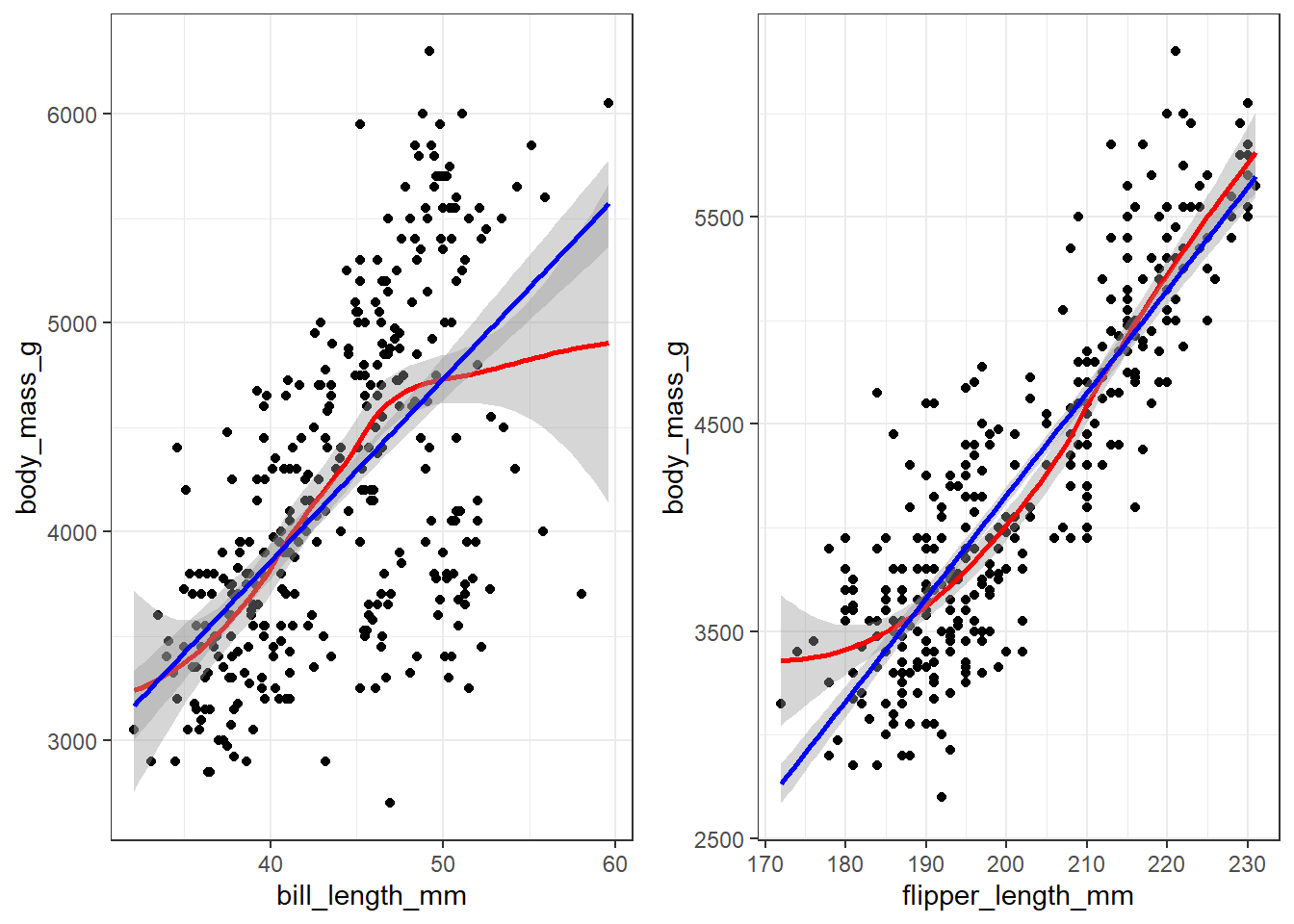
Both variables appear to have a mostly linear relationship with body mass. For penguins with bill length over 50mm the slope may decrease, but the data is sparse in the tails.
10.6.2 Normality of residuals.
There are two common ways to assess normality.
- A histogram or density plot with a normal distribution curve overlaid.
- A qqplot. This is also known as a ‘normal probability plot’. It is used to compare the theoretical quantiles of the data if it were to come from a normal distribution to the observed quantiles. PMA6 Figure 5.4 has more examples and an explanation.
gridExtra::grid.arrange(
  plot(check_normality(pen.bmg.model)),
  plot(check_normality(pen.bmg.model), type = "qq"),
  ncol=2
)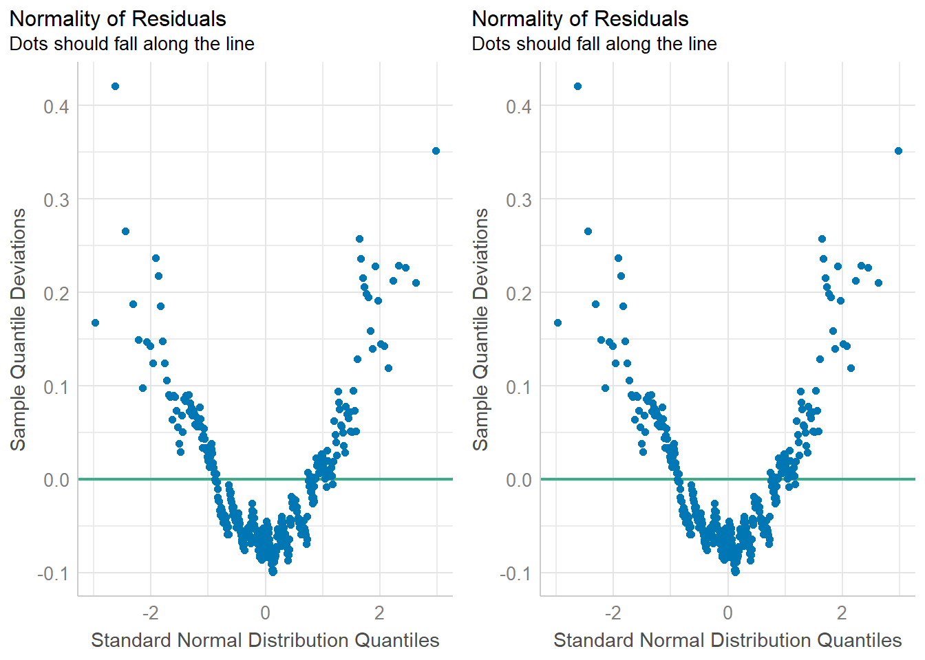
In both cases you want to assess how close the dots/distribution is to the reference curve/line.
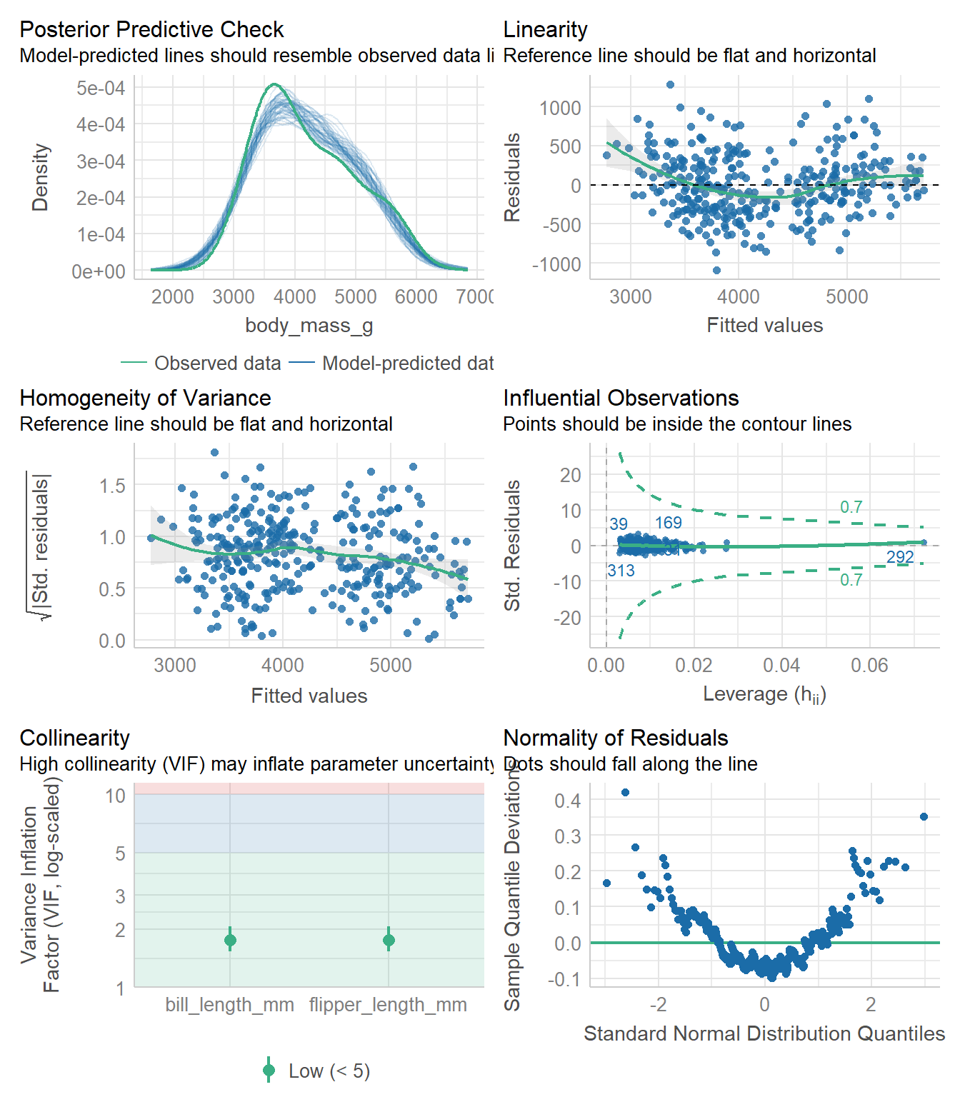
10.6.3 Homogeneity of variance
The variability of the residuals should be constant, and independent of the value of the fitted value \(\hat{y}\).
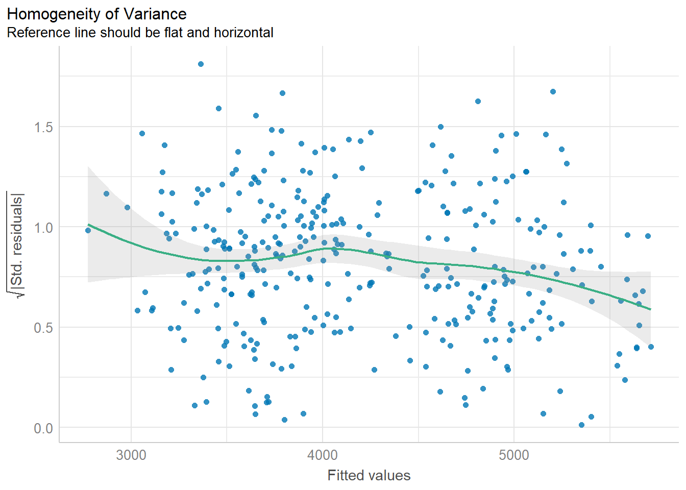
This assumption is often the hardest to be fully upheld. Here we see a slightly downward trend. However, this is not a massive violation of assumptions.