17.6 Including Covariates
A similar sort of shrinkage effect is seen with covariates included in the model.
Consider the covariate \(floor\), which takes on the value \(1\) when the radon measurement was read within the first floor of the house and \(0\) when the measurement was taken in the basement. In this case, county means are shrunk towards the mean of the response, \(log(radon)\), within each level of the covariate.
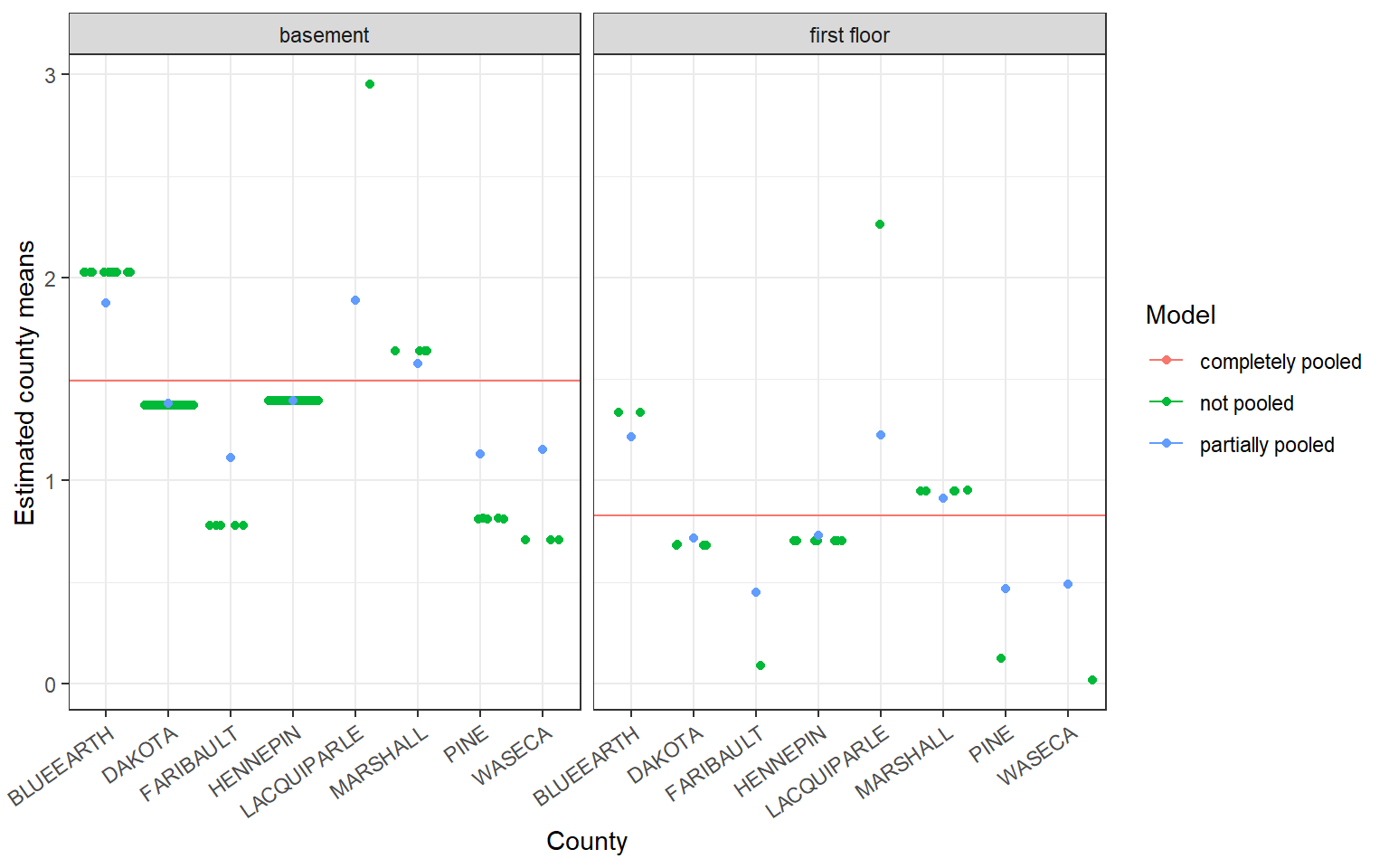
Covariates are fit using standard + notation outside the random effects specification, i.e. (1|county).
| log_radon | |||
|---|---|---|---|
| Predictors | Estimates | CI | p |
| (Intercept) | 1.49 | 1.40 – 1.59 | <0.001 |
| floor [first floor] | -0.66 | -0.80 – -0.53 | <0.001 |
| Random Effects | |||
| σ2 | 0.53 | ||
| τ00 county | 0.10 | ||
| ICC | 0.16 | ||
| N county | 85 | ||
| Observations | 919 | ||
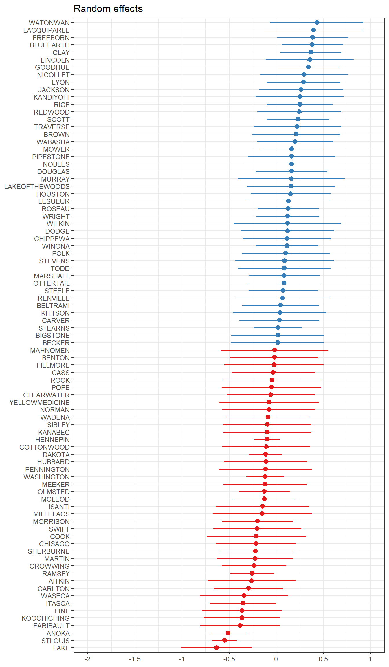
Note that in this table format, \(\tau_{00} = \sigma^{2}_{\alpha}\) and \(\sigma^{2} = \sigma^{2}_{\epsilon}\). The estimated random effects can also be easily visualized using functions from the sjPlot package.
Function enhancements –
- Display the fixed effects by changing
type="est". - Plot the slope of the fixed effect for each level of the random effect
sjp.lmer(ri.with.x, type="ri.slope")– this is being depreciated in the future but works for now. Eventually I’ll figure out how to get this plot out ofplot_model().