• Applied Statistics course notes
  • Preface
  • I Preparing Data for Analysis
  • 1 Workflow and Data Cleaning
    • 1.1 Generating a reproducible workflows
      • 1.1.1 Literate programming
      • 1.1.2 Reproducible Research + Literate Programming
    • 1.2 Import data
      • 1.2.1 Renaming variable names for sanity sake
    • 1.3 Data Management
      • 1.3.1 Missing data
      • 1.3.2 Identifying Variable Types
      • 1.3.3 Outliers
      • 1.3.4 Creating secondary variables
    • 1.4 Saving your changes
    • 1.5 Wide vs. Long data
    • 1.6 Dealing with missing data post-analysis
      • 1.6.1 Regression
      • 1.6.2 Factor Analysis and Principle Components
  • 2 Visualizing Data
    • 2.1 The syntax of ggplot
      • 2.1.1 Required arguments
      • 2.1.2 Optional but helpful arguments
    • 2.2 The Data
    • 2.3 Univariate Visualizations
      • 2.3.1 Categorical variables
      • 2.3.2 Continuous Measures
    • 2.4 Bivariate Visualizations
      • 2.4.1 Categorical v. Categorical
      • 2.4.2 Grouped bar charts with percentages
      • 2.4.3 Continuous v. Continuous
      • 2.4.4 Continuous v. Categorical
      • 2.4.5 Joy plots / Ridgelines
    • 2.5 Faceting / paneling
    • 2.6 Multiple plots per window
    • 2.7 Multivariate (3+ variables)
      • 2.7.1 Three continuous
      • 2.7.2 Scatterplot matrix
      • 2.7.3 Two categorical and one continuous
      • 2.7.4 Two continuous and one categorical
    • 2.8 Paneling on two variables
    • 2.9 Troubleshooting
    • 2.10 But what about…
      • 2.10.1 Other plots not mentioned
    • 2.11 Additional Resources
  • 3 Selecting Appropriate Analyses
  • II Statistical Inference
  • 4 Foundations for Inference
  • 5 Bivariate Analysis
    • 5.1 Assumption of Independent Observations
    • 5.2 Choosing appropriate bivariate analysis
    • 5.3 (Q~B) Two means: T-Test
      • 5.3.1 Assumptions
      • 5.3.2 Sampling Distribution for the difference
      • 5.3.3 Example: Smoking and BMI
    • 5.4 (Q~C) Multiple means: ANOVA
      • 5.4.1 Formulation of the One-way ANOVA model
      • 5.4.2 Analysis of Variance Table*:
      • 5.4.3 The F-distribution
      • 5.4.4 Assumptions
      • 5.4.5 Example: A comparison of plant species under low water conditions
      • 5.4.6 Coefficient of determination \(R^{2}\)
      • 5.4.7 Multiple Comparisons
    • 5.5 (C~C) Multiple Proportions: \(\chi^{2}\)
      • 5.5.1 Conditions for the sampling distribution to be normal.
      • 5.5.2 Example: Are Mammograms effective?
      • 5.5.3 Example: Smoking and General Health
      • 5.5.4 Multiple Comparisons
    • 5.6 (Q~Q) Correlation
      • 5.6.1 Strength of the correlation
      • 5.6.2 Example: Federal spending per capita and poverty rate
  • III Regression Modeling
  • 6 Introduction
    • 6.1 Opening Remarks
  • 7 Simple Linear Regression
    • 7.1 Example
      • 7.1.1 Caution on out of range predictions
    • 7.2 Mathematical Model
      • 7.2.1 Unifying model framework
    • 7.3 Parameter Estimates
      • 7.3.1 Sum of Squares
    • 7.4 Assumptions
    • 7.5 Example
    • 7.6 Model Diagnostics
    • 7.7 Prediction
      • 7.7.1 Predict the average value of Y (\(\hat{y}\)) based on the model
      • 7.7.2 Confidence intervals for the predicted mean
      • 7.7.3 Predict the average value of Y \((\hat{y_{i}})\) for a certain value of \(x^{*}\)
      • 7.7.4 Predict a new value of Y \(\hat{y_{i}}\) for a certain value of \(x^{*}\)
    • 7.8 ANOVA for regression
    • 7.9 Correlation Coefficient
  • 8 Moderation and Stratification
    • 8.1 Moderation
      • 8.1.1 Example 1: Simpson’s Paradox
      • 8.1.2 Example 2: Sepal vs Petal Length in Iris flowers
    • 8.2 Stratification
    • 8.3 Identifying a moderator
      • 8.3.1 What to look for in each type of analysis
    • 8.4 Example 2 (cont.) Correlation & Regression
    • 8.5 Example 3: ANOVA
    • 8.6 Example 4: Chi-Squared
  • 9 Multiple Linear Regression
    • 9.1 Mathematical Model
    • 9.2 Parameter Estimation
    • 9.3 Fitting the model
    • 9.4 Interpreting Coefficients
      • 9.4.1 Continuous predictors
      • 9.4.2 Binary predictors
      • 9.4.3 Categorical Predictors
    • 9.5 Presenting results
    • 9.6 Confounding
    • 9.7 What to watch out for
  • 10 Model Building
    • 10.1 Interactions
      • 10.1.1 Fitting interaction models & interpreting coefficients
      • 10.1.2 Categorical Interaction variables
      • 10.1.3 Example 2
      • 10.1.4 Example 3:
    • 10.2 Wald test
      • 10.2.1 Example: Modeling depression score
      • 10.2.2 Testing for a moderation effect in a multiple regression model.
    • 10.3 Multicollinearity
    • 10.4 Variable Selection Process
      • 10.4.1 Automated selection procedures
      • 10.4.2 LASSO Regression (PMA6 9.7)
    • 10.5 Comparing between models
      • 10.5.1 RSS: Residual Sum of Squares
      • 10.5.2 General F Test
      • 10.5.3 Likelihood function
      • 10.5.4 Multiple \(R^{2}\)
      • 10.5.5 Adjusted \(R^{2}\)
      • 10.5.6 Mallows \(C_{p}\)
      • 10.5.7 Akaike Information Criterion (AIC)
      • 10.5.8 Bayesian Information Criterion (BIC)
      • 10.5.9 AIC vs BIC
    • 10.6 Model Diagnostics
      • 10.6.1 Linearity
      • 10.6.2 Normality of residuals.
      • 10.6.3 Homogeneity of variance
      • 10.6.4 Posterior Predictions
      • 10.6.5 All at once
    • 10.7 General Advice (PMA6 9.9)
    • 10.8 What to watch out for (PMA6 9.10)
  • 11 Generalized Linear Models
    • 11.1 Fitting GLMs
      • 11.1.1 R
      • 11.1.2 SPSS
      • 11.1.3 Stata
    • 11.2 Binary outcome data
    • 11.3 Logistic Regression
      • 11.3.1 Interpreting Odds Ratios
      • 11.3.2 Confidence Intervals
      • 11.3.3 Example: The effect of gender on Depression
      • 11.3.4 Multiple Logistic Regression
      • 11.3.5 Effect of a k unit change
      • 11.3.6 Example: Predictors of smoking status
      • 11.3.7 Model Fit
    • 11.4 Log-linear models
      • 11.4.1 Example
    • 11.5 Count outcome data
    • 11.6 Categorical outcome data
  • 12 Classification of Binary outcomes
    • 12.1 Predicted Probabilities
    • 12.2 Distribution of Predicted probabilities
      • 12.2.1 Plotting predictions against covariates
    • 12.3 Predicted Class (outcome)
    • 12.4 Confusion Matrix
    • 12.5 Vocabulary terms
    • 12.6 ROC Curves
    • 12.7 Model Performance
  • IV Multivariate Analysis
  • 13 Introduction
  • 14 Principal Component Analysis
    • 14.1 When is Principal Components Analysis (PCA) used?
    • 14.2 Basic Idea - change of coordinates
    • 14.3 More Generally
    • 14.4 R commands
      • 14.4.1 Generating PC’s
      • 14.4.2 Viewing the amount of variance contained by each PC
      • 14.4.3 Vizualize Loadings
    • 14.5 Data Reduction
      • 14.5.1 Choosing \(m\)
    • 14.6 Standardizing
    • 14.7 Example
    • 14.8 Use in Multiple Regression
      • 14.8.1 Example: Modeling acute illness
    • 14.9 Things to watch out for
    • 14.10 Additional References
  • 15 Factor Analysis
    • 15.1 Introduction
      • 15.1.1 Latent Constructs
      • 15.1.2 Comparison with PCA
      • 15.1.3 EFA vs CFA
    • 15.2 Factor Model
      • 15.2.1 Components of Variance
      • 15.2.2 Two big steps
    • 15.3 Example data setup
    • 15.4 Factor Extraction Methods
      • 15.4.1 Principal components (PC Factor model)
      • 15.4.2 Iterated components
      • 15.4.3 Maximum Likelihood
      • 15.4.4 Uniqueness
      • 15.4.5 Resulting factors
    • 15.5 Rotating Factors
      • 15.5.1 Varimax Rotation
      • 15.5.2 Oblique rotation
    • 15.6 Factor Scores
    • 15.7 What to watch out for
    • 15.8 Additional Resources
  • V Multi-level Modeling
  • 16 Introduction
    • 16.1 Example School Data
    • 16.2 Multi-level models
  • 17 Random Intercept Models
    • 17.1 Pooling
    • 17.2 Mathematical Models
      • 17.2.1 Complete Pooling
      • 17.2.2 No Pooling
      • 17.2.3 Partial Pooling (RI)
    • 17.3 Components of Variance
    • 17.4 Fitting models in R
      • 17.4.1 Comparison of estimates
    • 17.5 Estimation Methods
    • 17.6 Including Covariates
    • 17.7 More Random Effects
    • 17.8 Centering terms
      • 17.8.1 A generic dplyr approach to centering.
    • 17.9 Specifying Correlation Structures
      • 17.9.1 Changing covariance structures in R
    • 17.10 Additional References
      • 17.10.1 Lecture notes from other classes found on the interwebs
      • 17.10.2 Package Vignettes
  • VI Other Topics
  • 18 Missing Data
    • 18.1 Identifying missing data
      • 18.1.1 Visualize missing patterns
    • 18.2 Effects of Nonresponse
    • 18.3 Missing Data Mechanisms
      • 18.3.1 Demonstration via Simulation
    • 18.4 General strategies
      • 18.4.1 Complete cases analysis
      • 18.4.2 Available-case analysis
      • 18.4.3 Imputation
    • 18.5 Imputation Methods
    • 18.6 Multiple Imputation (MI)
      • 18.6.1 Goals
      • 18.6.2 Technique
      • 18.6.3 MI as a paradigm
      • 18.6.4 Inference on MI
    • 18.7 Multiple Imputation using Chained Equations (MICE)
      • 18.7.1 Overview
      • 18.7.2 Process / Algorithm
      • 18.7.3 Convergence
      • 18.7.4 Imputation Methods
    • 18.8 Diagnostics
    • 18.9 Example: Prescribed amount of missing.
      • 18.9.1 Multiply impute the missing data using mice()
      • 18.9.2 Check the imputation method used on each variable.
      • 18.9.3 Check Convergence
      • 18.9.4 Look at the values generated for imputation
      • 18.9.5 Create a complete data set by filling in the missing data using the imputations
      • 18.9.6 Visualize Imputations
      • 18.9.7 Calculating bias
    • 18.10 Post MICE data management
    • 18.11 Final thoughts
    • 18.12 Additional References
  • VII APPENDIX
  • 19 Setup R & RStudio
    • 19.1 ⚠️ Before you begin
    • 19.2 Download and install R
      • 🔽 Download R v 4.1+
      • ✏️ Install
      • 🎦 Video Tutorials for both R and R Studio.
    • 19.3 Download and install R Studio
    • 19.4 Navigating RStudio
    • 19.5 Setting preferences
    • 19.6 Installing packages
      • 19.6.1 Common packages used in this notebook
    • 19.7 Organization using R Projects
    • 19.8 Literate programming with Quarto
      • 19.8.1 Creating PDF’s
    • 19.9 Seeking Help
      • 19.9.1 Advice on asking for help
      • 19.9.2 Help from inside R Studio
      • 19.9.3 Other Online
      • 19.9.4 Written
    • 19.10 Saving and closing your work.
      • 19.10.1 Restart R
    • 19.11 Acknowledgements
  • View source on Github

Applied Statistics

19.4 Navigating RStudio

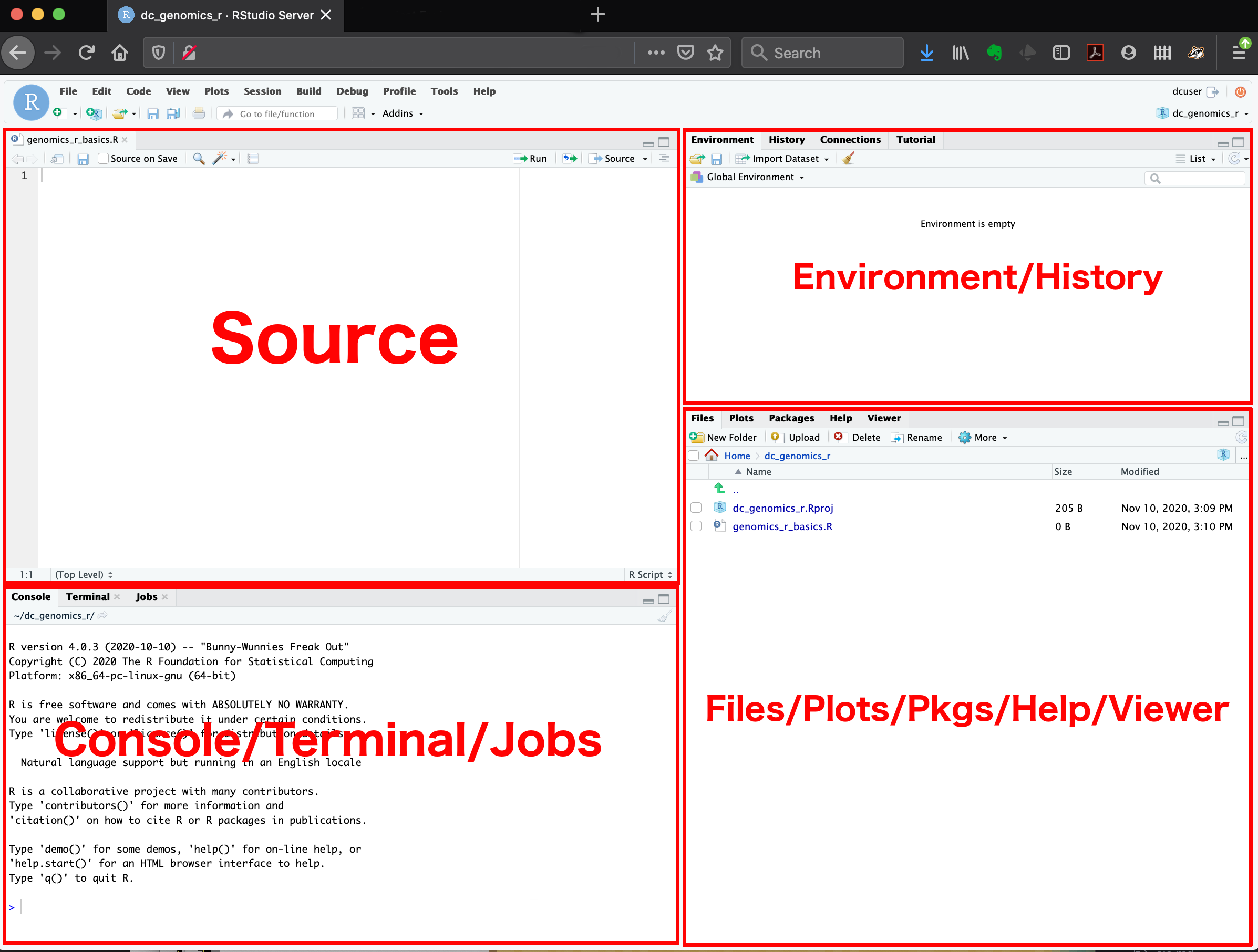
The major windows (or panes) of the RStudio environment:
  • Source: This pane is where you will write/view R scripts. Some outputs (such as if you view a dataset using View()) will appear as a tab here.
  • Console/Terminal/Jobs: This is actually where you see the execution of commands. This is the same display you would see if you were using R at the command line without RStudio. You can work interactively (i.e. enter R commands here), but for the most part we will run a script (or lines in a script) in the source pane and watch their execution and output here. The “Terminal” tab give you access to the BASH terminal (the Linux operating system, unrelated to R). RStudio also allows you to run jobs (analyses) in the background. This is useful if some analysis will take a while to run. You can see the status of those jobs in the background.
  • Environment/History: Here, RStudio will show you what datasets and objects (variables) you have created and which are defined in memory. You can also see some properties of objects/datasets such as their type and dimensions. The “History” tab contains a history of the R commands you’ve executed R.
  • Files/Plots/Packages/Help/Viewer: This multipurpose pane will show you the contents of directories on your computer. You can also use the “Files” tab to navigate and set the working directory. The “Plots” tab will show the output of any plots generated. In “Packages” you will see what packages are actively loaded, or you can attach installed packages. “Help” will display help files for R functions and packages. “Viewer” will allow you to view local web content (e.g. HTML outputs).

this page pulled directly from the Data Carpentry Genomics lesson