14.6 Factor Scores

• Can be used as dependent or independent variables in other analyses
• Each \(X\) is a function of \(F\)’s
• Factor Scores are the reverse: Each \(F\) is a function of the \(X\)’s
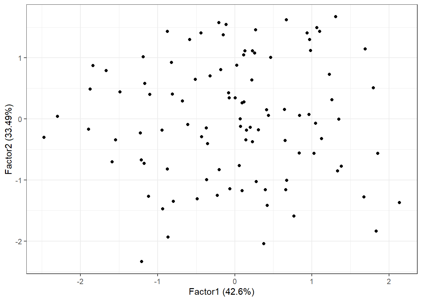
• Can be generated by adding the scores="regression" option to factanal(), or scores=TRUE in principal()
• Each record in the data set with no missing data will have a corresponding factor score.
  • principal() also has a missing argument that if set to TRUE it will impute missing values.

fa.ml.varimax <- factanal(stan.dta, factors=2, rotation="varimax", scores="regression")
summary(fa.ml.varimax$scores)
##     Factor1            Factor2        
##  Min.   :-2.32732   Min.   :-2.79312  
##  1st Qu.:-0.72413   1st Qu.:-0.54362  
##  Median : 0.09196   Median :-0.02376  
##  Mean   : 0.00000   Mean   : 0.00000  
##  3rd Qu.: 0.70603   3rd Qu.: 0.65339  
##  Max.   : 2.43371   Max.   : 2.18992
head(fa.ml.varimax$scores)
##          Factor1      Factor2
## [1,] -1.49174313  0.003612941
## [2,] -0.26254721  1.090864733
## [3,]  0.55516045  0.631119886
## [4,] -1.21028676 -1.281240452
## [5,] -0.04852211 -1.575691468
## [6,] -0.53768770  0.661138335

#library(ggforitfy)
autoplot(fa.ml.varimax) # see vignette for more info. Link at bottom

To merge these scores back onto the original data set providing there is no missing data you can use the bind_cols() function in dplyr.

data.withscores <- bind_cols(data, data.frame(fa.ml.varimax$scores))
kable(head(data.withscores))

X1	X2	X3	X4	X5	Factor1	Factor2
-0.8236763	-0.1210726	-0.5970760	-1.4752693	-1.2355056	-1.4917431	0.0036129
1.4013214	1.0733569	0.7681035	-0.0509857	0.0180061	-0.2625472	1.0908647
0.2781468	0.7574632	0.6445954	0.6765583	0.7532815	0.5551604	0.6311199
0.1819544	-1.3228227	-1.0847105	-0.9574722	-1.3719843	-1.2102868	-1.2812405
-1.6147171	-1.4254411	0.3519605	-0.0124497	-0.2523487	-0.0485221	-1.5756915
0.8251470	0.6245702	-1.2923348	-0.6345633	-0.0885945	-0.5376877	0.6611383