7.2 Mathematical Model
The mathematical model that we use for regression has three features.
- \(Y\) values are normally distributed at any given \(X\)
- The mean of \(Y\) values at any given \(X\) follows a straight line \(Y = \beta_{0} + \beta_{1} X\).
- The variance of \(Y\) values at any \(X\) is \(\sigma^2\) (same for all X). This is known as homoscedasticity, or homogeneity of variance.
Mathematically this is written as:
\[ Y|X \sim N(\mu_{Y|X}, \sigma^{2}) \\ \mu_{Y|X} = \beta_{0} + \beta_{1} X \\ Var(Y|X) = \sigma^{2} \]
and can be visualized as:
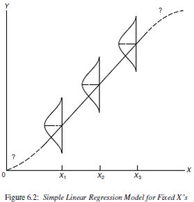
Figure 6.2
7.2.1 Unifying model framework
The mathematical model above describes the theoretical relationship between \(Y\) and \(X\). So in our unifying model framework to describe observed data,
DATA = MODEL + RESIDUAL
Our observed data values \(y_{i}\) can be modeled as being centered on \(\mu_{Y|X}\), with normally distributed residuals.
\[ y_{i} = \beta_{0} + \beta_{1} X + \epsilon_{i} \\ \epsilon_{i} \sim N(0, \sigma^{2}) \]