1.7 Identifying Outliers
Let’s look at the age variable in the depression data set.
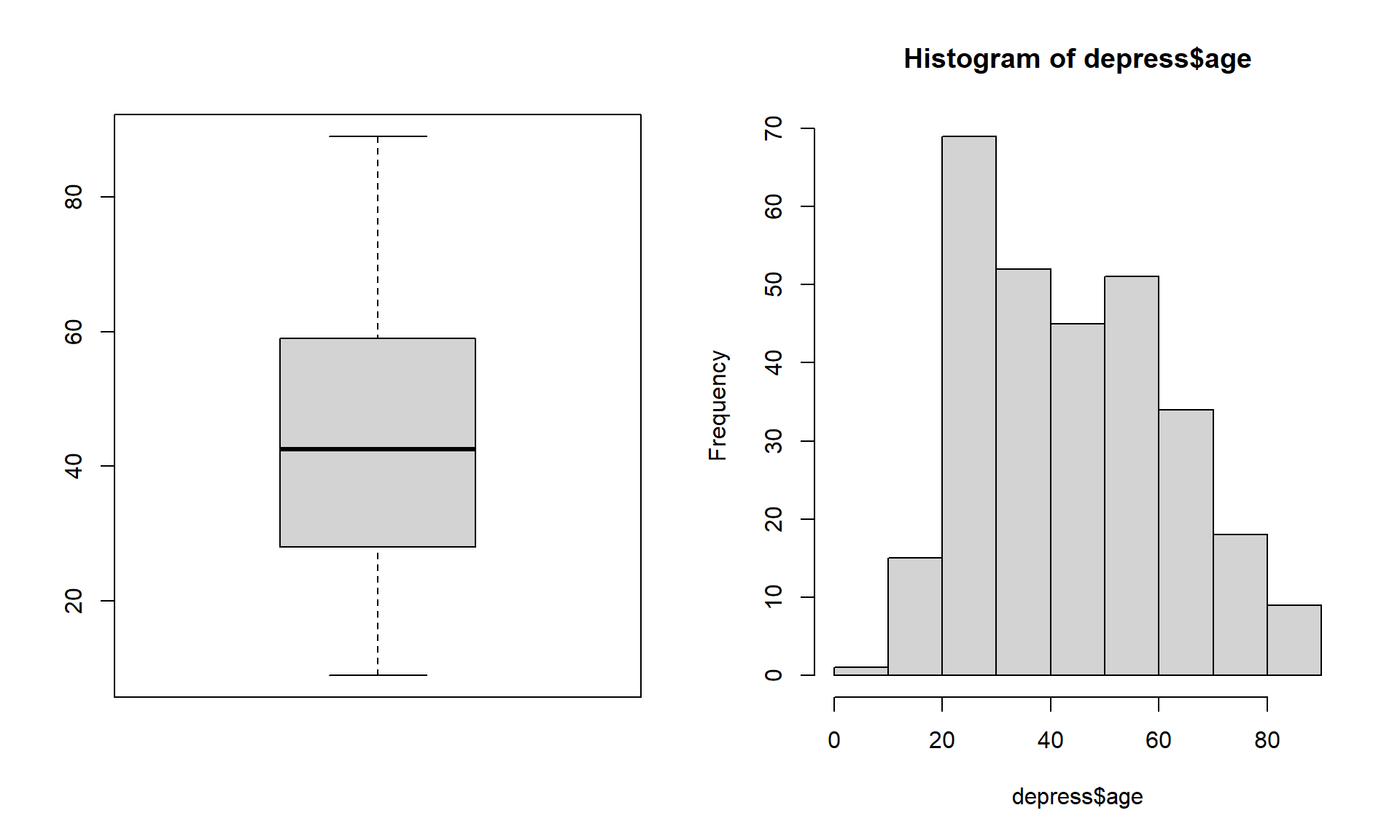
Just looking at the data graphically raises no red flags. The boxplot shows no outlying values and the histogram does not look wildly skewed. This is where knowledge about the data set is essential. The codebook does not provide a valid range for the data, but the description of the data starting on page 3 in the textbook clarifies that this data set is on adults. In the research world, this specifies 18 years or older.
Now look back at the graphics. See anything odd? It appears as if the data go pretty far below 20, possibly below 18. Let’s check the numerical summary to get more details.
The minimum value is a 9, which is outside the range of valid values for this variable. This is where you, as a statistician, data analyst or researcher goes back to the PI and asks for advice. Should this data be set to missing, or edited in a way that changes this data point into a valid piece of data.
Another example
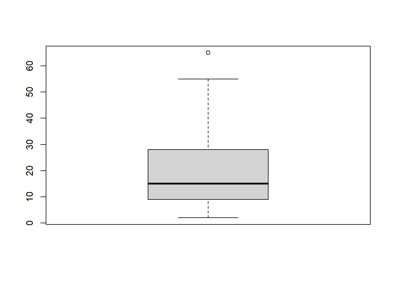
While there is at least one potential outliers (denoted by the dots), there are none so far away from the rest of the group (or at values such as 99 or -99 that may indicate missing codes) that we need to be concerned about.