14.4 Generating PC’s using R

Corresponding reading: PMA6 Ch 14.3-14.4

Calculating the principal components in R can be done using the function prcomp() and princomp(). This section of notes uses princomp(), not for any specific reason. STHDA has a good overview of the difference between prcomp() and princomp(). It appears that prcomp() may have some more post-analysis fancy visualizations available.

• Requirements of data: This must be a numeric matrix. Since I made up this example by generating data in section 14.2, I know they are numeric.

pr <- princomp(data)
summary(pr)
## Importance of components:
##                            Comp.1    Comp.2
## Standard deviation     11.4019265 4.2236767
## Proportion of Variance  0.8793355 0.1206645
## Cumulative Proportion   0.8793355 1.0000000

• The summary output above shows the first PC (Comp.1) explains the highest proportion of variance.
• The values for the matrix \(\mathbf{A}\) is contained in pr$loadings.

pr$loadings
## 
## Loadings:
##    Comp.1 Comp.2
## X1  0.854  0.519
## X2  0.519 -0.854
## 
##                Comp.1 Comp.2
## SS loadings       1.0    1.0
## Proportion Var    0.5    0.5
## Cumulative Var    0.5    1.0

To visualize these new axes, we plot the centered data.

a <- pr$loadings
x1 <- with(data, X1 - mean(X1))
x2 <- with(data, X2 - mean(X2))

plot(c(-40, 40), c(-20, 20), type="n",xlab="x1", ylab="x2")
points(x=x1, y=x2, pch=16)
abline(0, a[2,1]/a[1,1]); text(30, 10, expression(C[1]))
abline(0, a[2,2]/a[1,2]); text(-10, 20, expression(C[2]))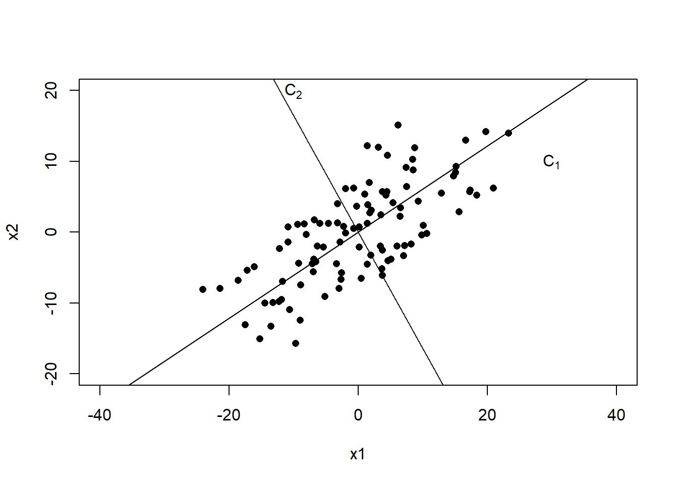

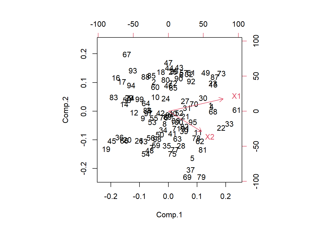
Plot the original data on the new axes we see that PC1 and PC2 are uncorrelated. The red vectors show you where the original coordinates were at.

biplot(pr)