Load Libraries

library(scales); library(dplyr); library(gridExtra); 
library(xtable); library(magrittr); library(knitr)
library(vcd)
opts_chunk$set(echo = TRUE, warning=FALSE, message=FALSE, cache=TRUE)

Helper functions

univ.n.p <- function(df, var, dig){
  df %>% select_(var) %>% na.omit() %>% group_by_(var) %>% 
    summarise(n=n()) %>% 
    mutate(pct=round(n/sum(n),dig))
}

univ.n.pct <- function(df, var){
  df %>% select_(var) %>% na.omit() %>% group_by_(var) %>% 
    summarise(n=n()) %>% 
    mutate(pct=paste0(round(n/sum(n)*100,1), '%'))
}

biv.n.col.p <- function(df, row.var, col.var) {
  df %>% group_by_(row.var, col.var) %>% 
    summarise(count=n()) %>%
    mutate(pct=round(count/sum(count),3))
}

Load & prepare data

data.path <- "data6e/"

raw <- read.delim(paste0(data.path,"Parhiv.txt"), sep="\t", header=TRUE)

parhiv <- raw %>% 
  mutate(JOBMO = factor(JOBMO, 
                        labels=c("Employed", "Unemployed", "Retired/Disabled")), 
         EDUMO = factor(EDUMO, 
                        labels=c("Less than High School", "High School Graduate/GED", 
                                 "Post Secondary")),
         bsi_overall = rowMeans(raw[,grep("BSI", names(raw))]), 
         log_bsi_overall = log(bsi_overall+.01), 
         parent_bonding = (PB01+(4-PB02)+(4-PB04)+PB05+PB06+
                           PB11+PB12+(4-PB14)+(4-PB16)+PB17+(4-PB18)+(4-PB24))/12)
parhiv$AGEALC[parhiv$AGEALC==0] <- NA
parhiv$AGEMAR[parhiv$AGEMAR==0] <- NA
parhiv$AGESMOKE[parhiv$AGESMOKE==0] <- NA

raw.d <- read.delim(paste0(data.path,"Depress.txt"), sep="\t", header=TRUE)
depress <- raw.d %>% 
  mutate(gender = factor(SEX, 
                         labels=c("Male", "Female")), 
         educat =  factor(EDUCAT, 
                         labels=c("<HS", "Some HS", "HS Grad", "Some college", 
                                  "BS", "MS", "PhD")), 
         marital = factor(MARITAL, 
                         labels = c("Never Married", "Married", "Divorced", 
                                    "Separated", "Widowed")))

raw.l <- read.delim(paste0(data.path,"Lung.txt"), sep="\t", header=TRUE)

mice <- read.delim(paste0(data.path,"Mice.txt"), sep="\t", header=TRUE)

Demo

hist(parhiv$bsi_overall);box()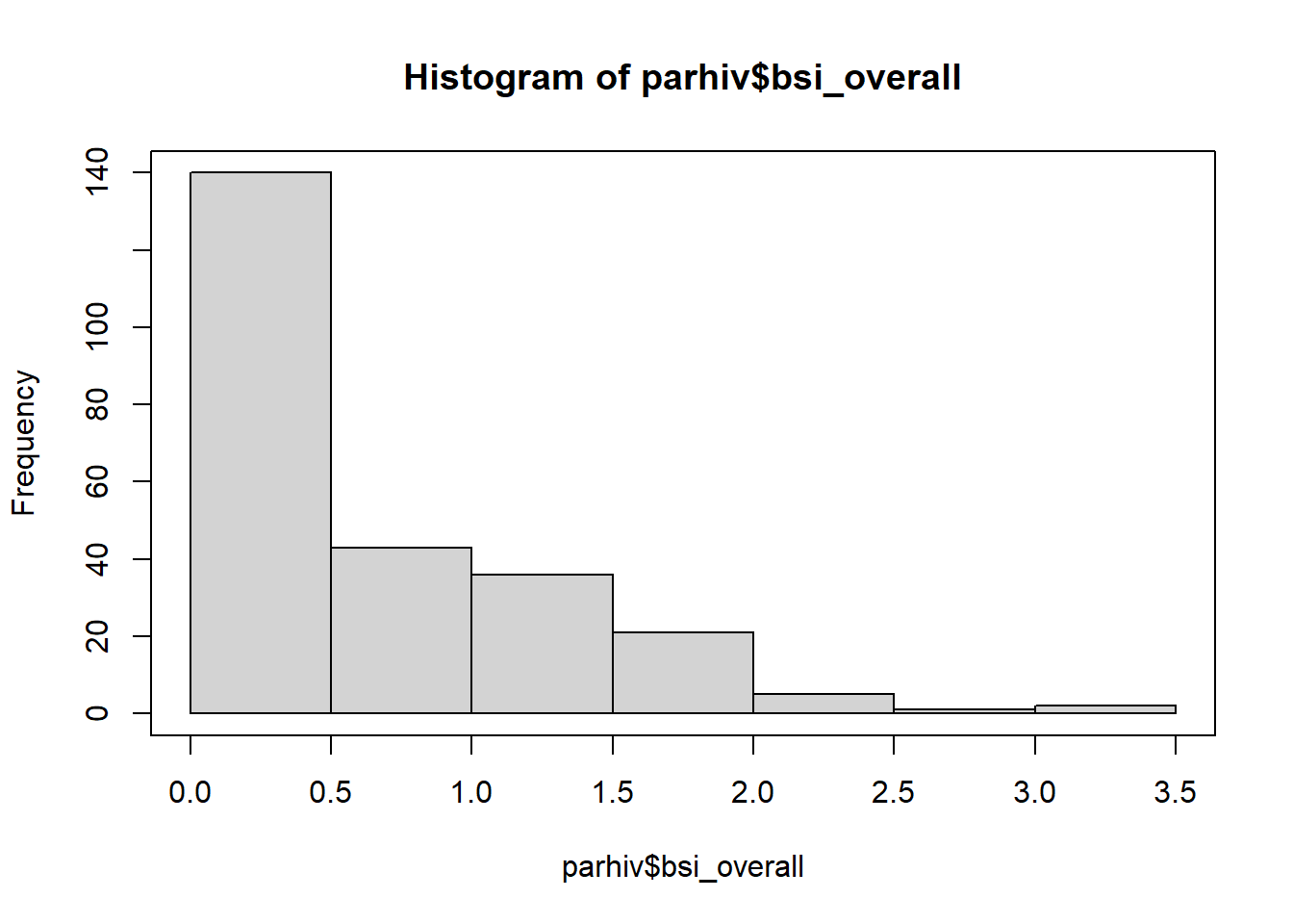

ggplot(parhiv, aes(x=bsi_overall)) + 
  geom_histogram() +
  theme_bw(base_size=16)

ggplot(parhiv, aes(x=bsi_overall)) + 
  geom_histogram() + 
  theme_classic(base_size = 20) + 
  xlab("BSI score") + ylab("Frequency") + ggtitle("Brief Symptom Inventory Score")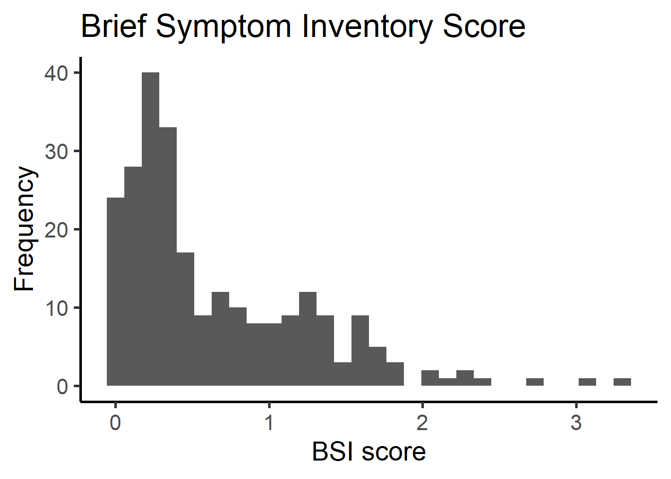

Univariate

Categorical

Univariate barplot with counts

ggplot(filter(parhiv, !is.na(EDUMO)), aes(x=EDUMO)) + 
  theme_classic(base_size = 20) + 
  geom_bar(aes(y = ..count..)) + ggtitle("Frequency of educational level") + 
  xlab("Highest educational level attained") +
  scale_x_discrete(labels = function(x) lapply(strwrap(x, width = 12, simplify = FALSE), 
                                               paste, collapse="\n")) + 
  geom_text(aes(y=..count.. + 5, label=..count..), stat='count', size = 7) + 
  theme(axis.ticks.x=element_blank())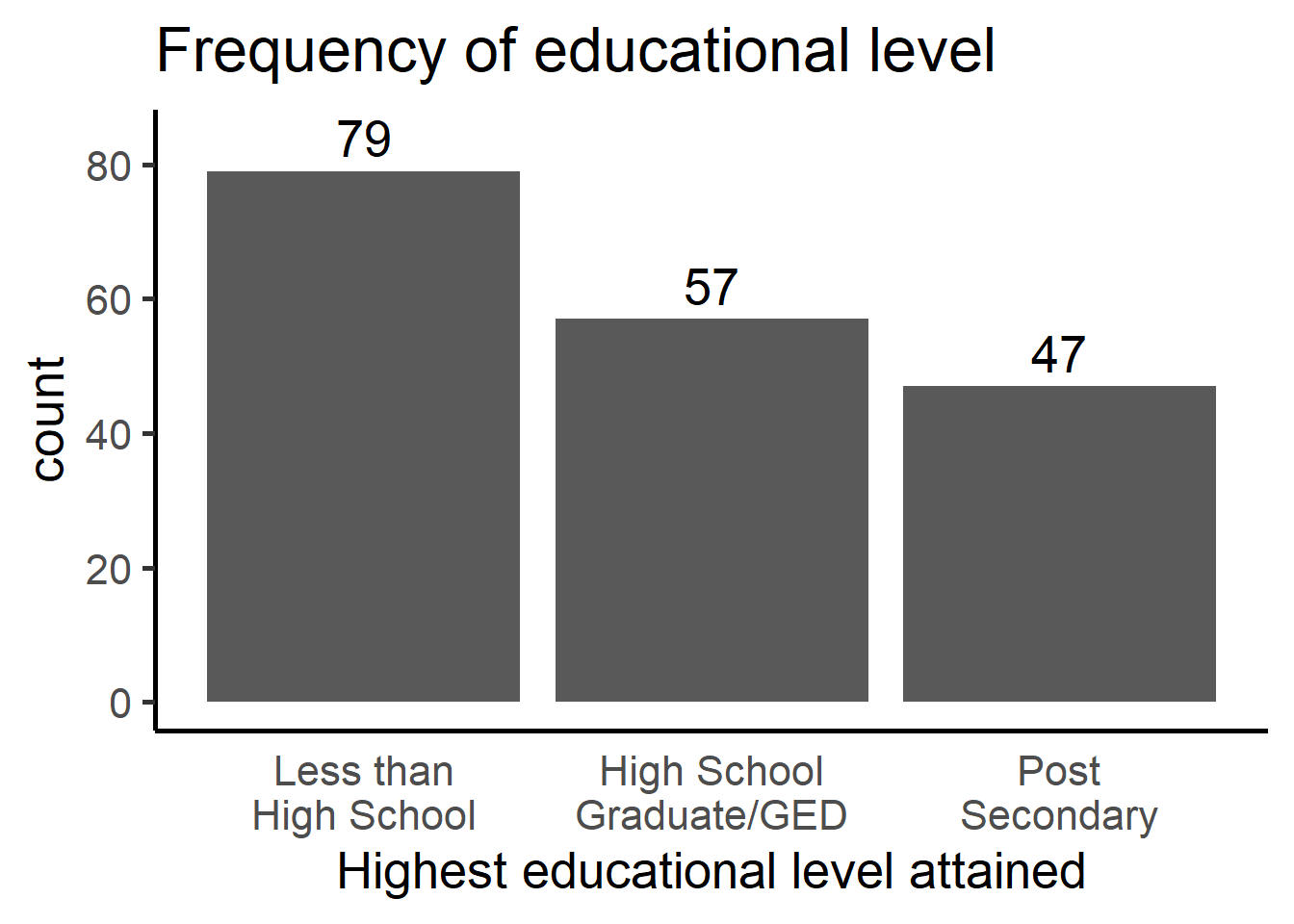

Univariate barplot with percentages

ptab.ctp <- univ.n.p(parhiv, "EDUMO", dig=3)

ggplot(ptab.ctp, aes(x=EDUMO)) + 
  geom_bar(aes(y=pct), stat="identity") + 
  xlab("Highest educational level attained") + ylab("") + 
  ggtitle("Percent of mothers with each \n educational level") + 
  theme_classic(base_size = 20) + 
  scale_y_continuous(labels=percent, limits=c(0,1)) + ylab("") + 
  scale_x_discrete(labels = function(x) lapply(strwrap(x, width = 12, simplify = FALSE), 
                                               paste, collapse="\n")) + 
  geom_text(aes(y=pct + .05, label=paste0(pct*100, "%")), size = 7) + 
  theme(axis.ticks.x=element_blank())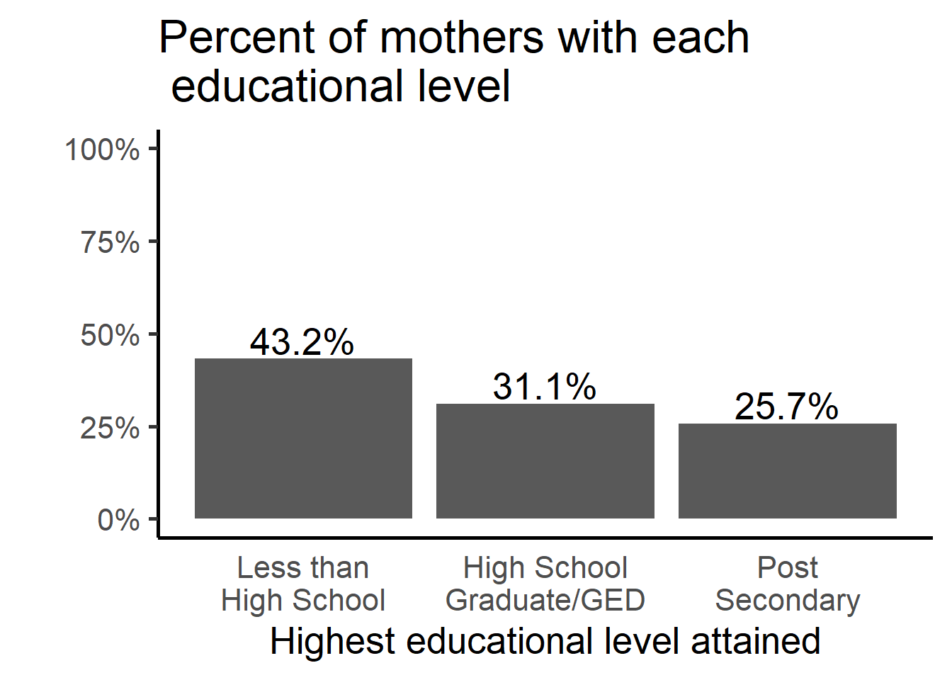

Cleveland Dotplot

ptab.empl <- univ.n.pct(depress, "marital")

ggplot(ptab.empl, aes(x=n, y=reorder(marital, n), label=n)) +  
  geom_point(size = 3) + 
  geom_text(size=5, vjust=-1) + 
  xlab("Frequency") + ylab("Marital Status") + ggtitle("Frequency of marital status") +
  theme_classic(base_size=20) + 
  scale_x_continuous(limits=c(0,130))+
  theme(panel.grid.major.x = element_blank(), axis.ticks.y=element_blank(),
        panel.grid.minor.x = element_blank(),
        panel.grid.major.y = element_line(color='grey60', linetype='dashed'))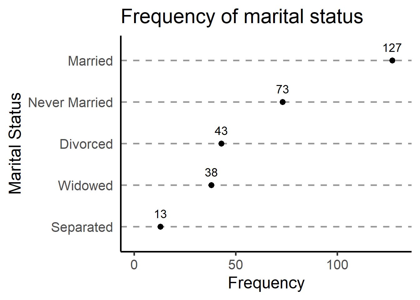

Pie Chart

dc <- table(depress$marital)

pie(dc, labels = paste0(names(dc), ' (', round(prop.table(dc)*100,1), "%)"), 
    col = c("#f7f7f7","#cccccc", "#969696", "#636363", "#252525"), cex=1.5, radius=0.5)

Stem-leaf plot

par(mar=c(0,0,0,0), oma=c(0,0,0,0))
plot(c(0,0.5), c(0,1), type="n", axes=FALSE, main="", ylab="", xlab="")
tmp <- capture.output(stem(sort(depress$AGE)))
tmp <- tmp[4:length(tmp)]
text(0,1, paste(tmp, collapse='\n'), adj=c(0,1), family='mono', cex=1)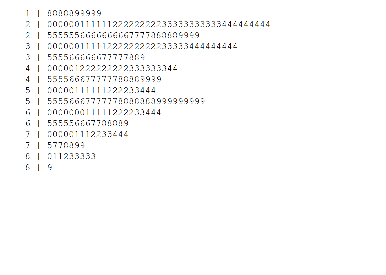

Stripchart

ggplot(depress, aes(y=AGE, x=1)) + 
  geom_jitter(position = position_jitter(0.2)) + 
  ylab("Age") + 
  scale_x_continuous(limits=c(0,2)) +  
  theme_classic(base_size=20)+ xlab("")+
  theme(panel.grid.major.y = element_blank(), axis.ticks.y=element_blank(),
        panel.grid.minor.y= element_blank(), axis.text.y=element_blank()) + 
  coord_flip()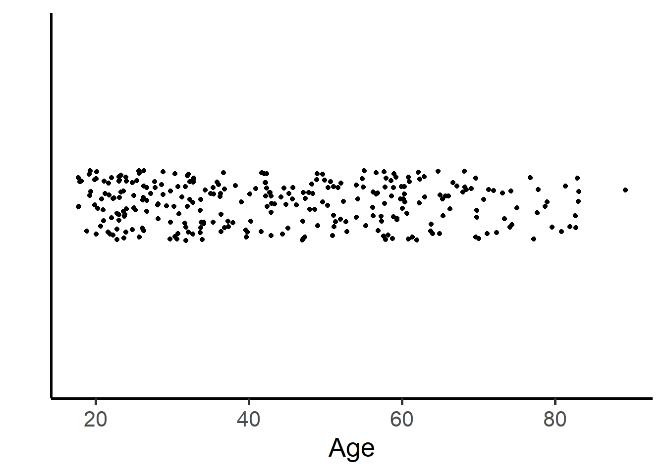

Continuous

Univariate histogram

ggplot(depress, aes(x=AGE)) + 
  geom_histogram(colour="black", fill="grey80", binwidth=10) +  
  xlab("Age") + ylab("Frequency") + 
  ggtitle("Distribution of age") + 
  theme_classic(base_size = 16) +
  scale_x_continuous(limits=c(20,80), breaks=seq(20,80,by=10))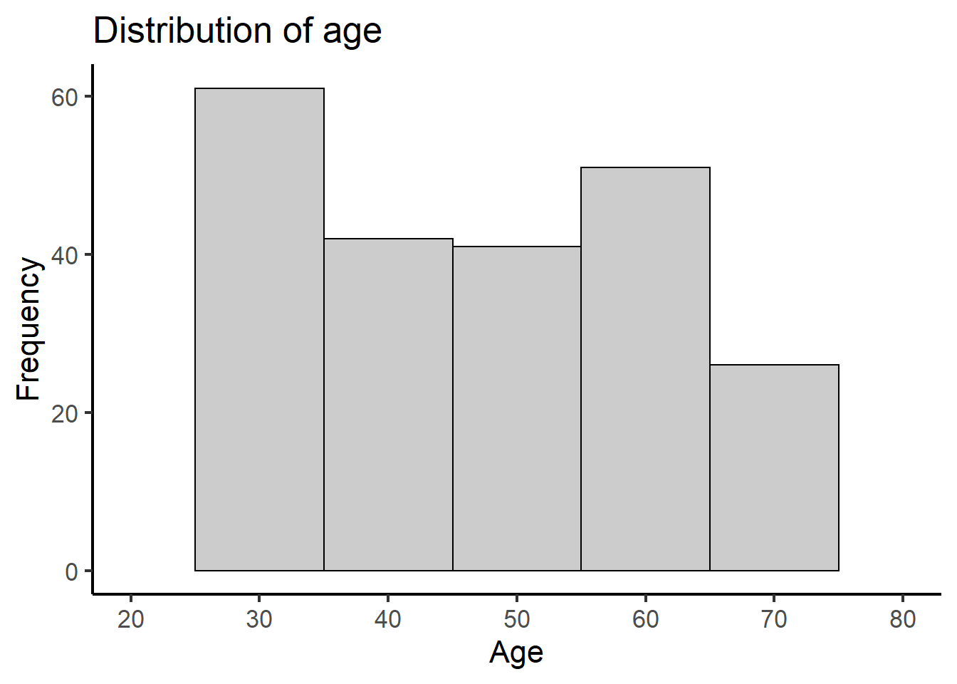

Univariate histogram with default bins

ggplot(depress, aes(x=AGE)) + 
  geom_histogram(colour="black", fill="grey80") + 
  xlab("Age") + ylab("Frequency") + 
  ggtitle("Distribution of age") + 
  theme_classic(base_size = 16) +
  scale_x_continuous(limits=c(15,90), breaks=seq(20,90,by=10))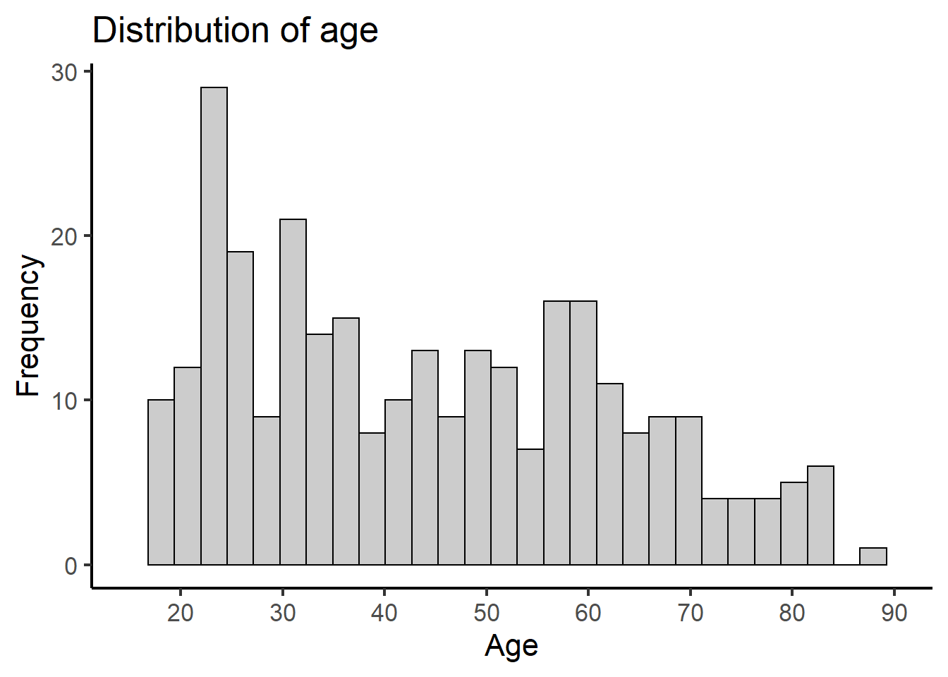

Univariate Density

ggplot(depress, aes(x=AGE)) + 
  geom_histogram(aes(y=..density..), colour="black", fill="grey80") +  
  xlab("Age") + ylab("Density") + 
  geom_density(colour="black", lwd=1.1) + 
  scale_x_continuous(limits=c(15,90), breaks=seq(20,90,by=10)) + 
  ggtitle("Distribution of age") + theme_classic(base_size = 16)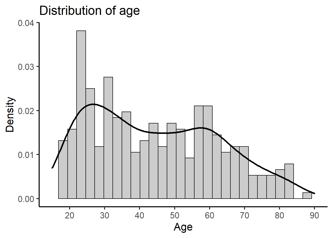

Univariate boxplot

txt <- boxplot(depress$AGE, plot=FALSE)$stats
data.labels <- data.frame(value=as.vector(txt), lab=as.character(txt))
labels <- data.frame(value=as.vector(txt), 
                     lab=c("Min", "Q(0.25)", "Median", "Q(0.75)", "Max"))

ggplot(depress, aes(y=AGE, x=1)) + 
  geom_boxplot(width=.3) + ylab("Age") + xlab("") + 
  scale_x_continuous(limits=c(0.5,1.35)) + 
  theme_classic(base_size = 16) +
  theme(axis.ticks = element_blank(), axis.text.x = element_blank()) + 
  geom_text(data=data.labels,aes(x=0.75,y=value,label=lab),angle=0, size=5) + 
  geom_text(data=labels,aes(x=0.6,y=value,label=lab),angle=0, size=5)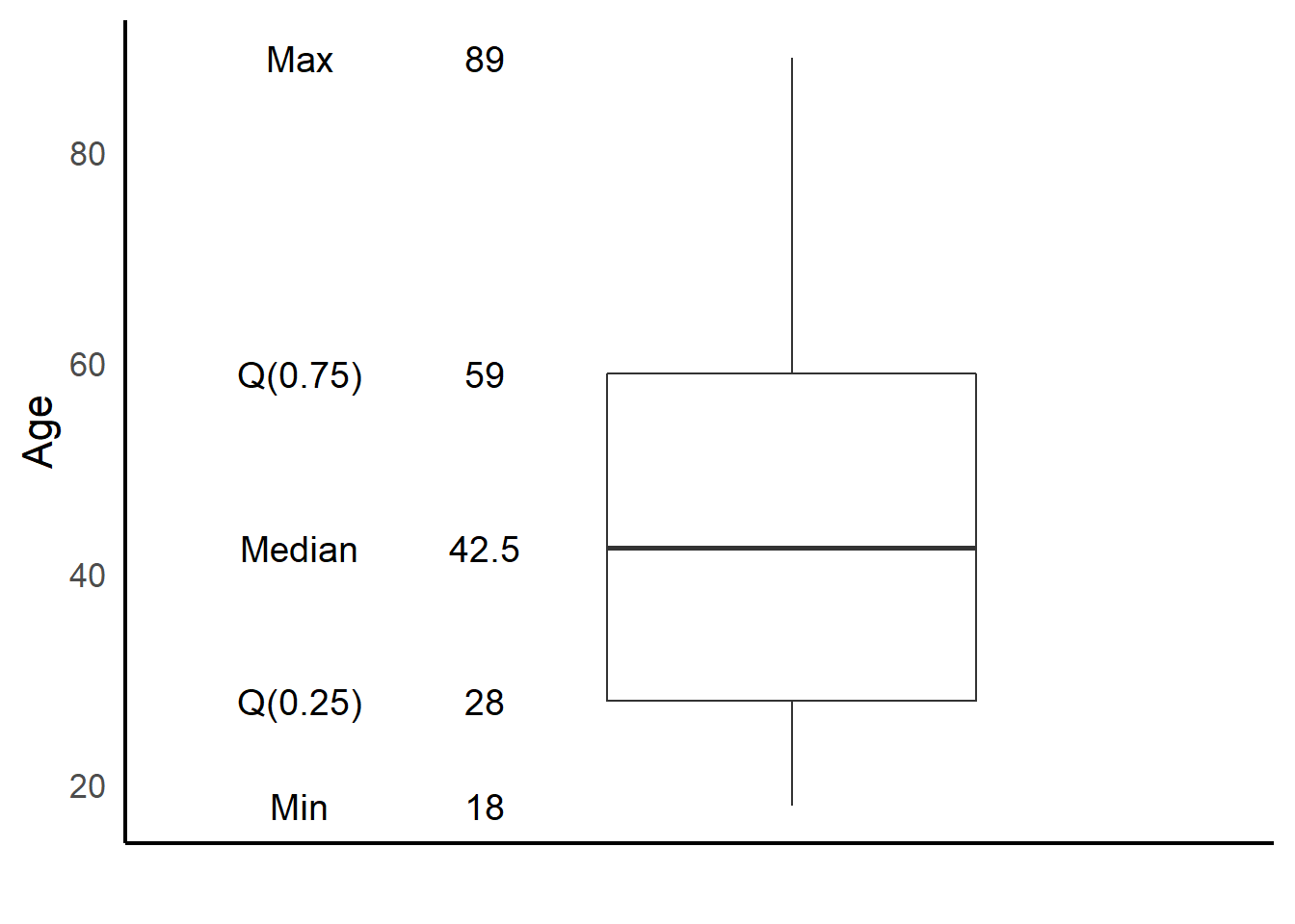

Univariate boxplot modified

txt <- boxplot(depress$CESD, plot=FALSE)$stats
data.labels <- data.frame(value=as.vector(txt), lab=as.character(txt))
labels <- data.frame(value=as.vector(txt), 
                     lab=c("Min", "Q(0.25)", "Median", "Q(0.75)", "Largest value \n within fence"))

ggplot(depress, aes(y=CESD, x=1)) + 
  geom_boxplot(width=.3) + ylab("CESD") + xlab("") + 
  scale_x_continuous(limits=c(0.75,1.5)) + 
  theme_classic(base_size = 16) + 
  theme(axis.ticks = element_blank(), axis.text.x = element_blank()) + 
  geom_text(data=data.labels,aes(x=1.25,y=value,label=lab),angle=0, size=5) + 
  geom_text(data=labels,aes(x=1.4,y=value,label=lab),angle=0, size=5)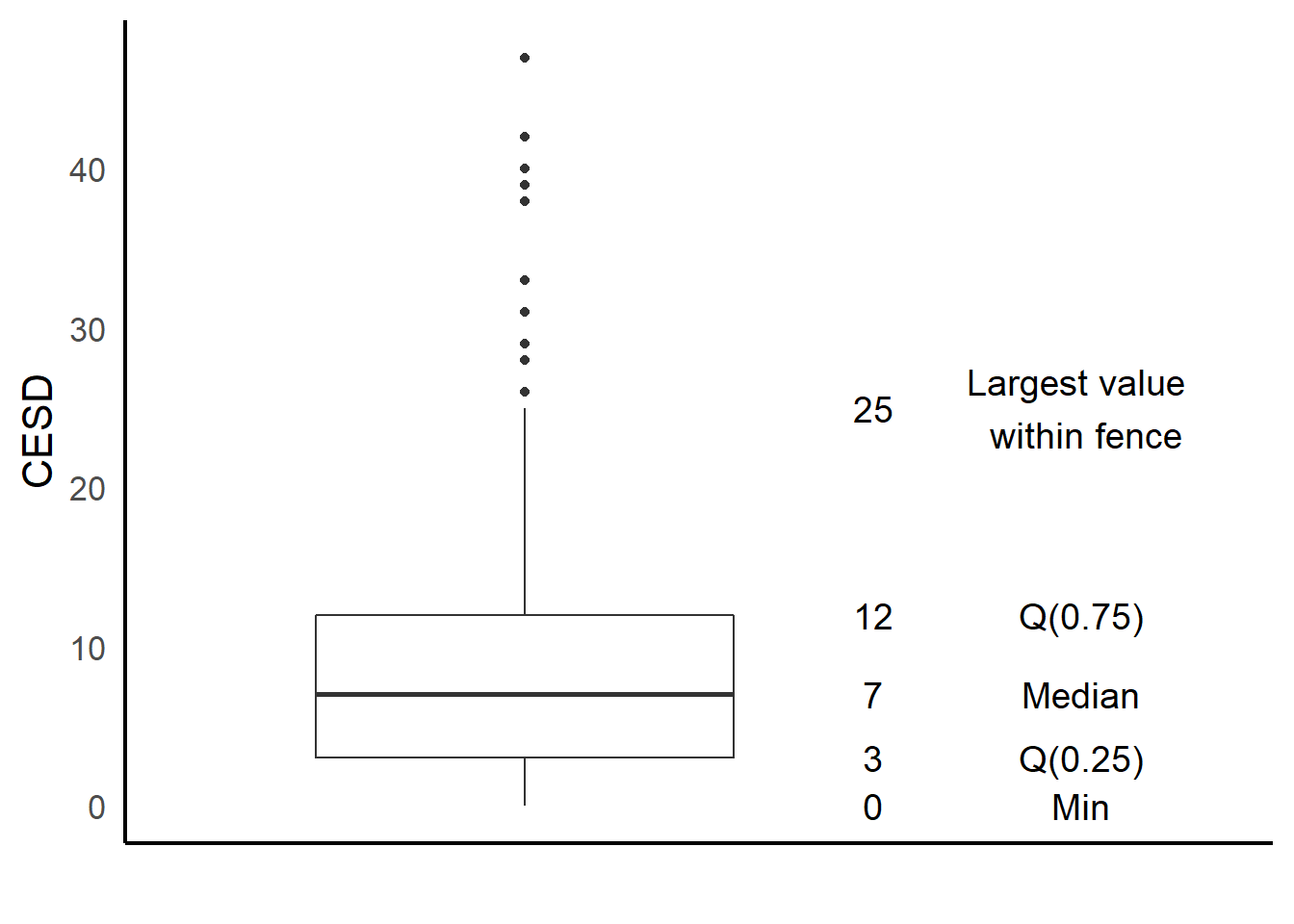

Univariate boxplot

ggplot(depress, aes(y=AGE, x=1)) + 
  geom_boxplot(width=.3) + geom_violin(alpha=.2) +
  ylab("Age") + xlab("") + theme_classic(base_size = 16) + 
  theme(axis.ticks = element_blank(), axis.text.x = element_blank()) + 
  stat_summary(fun.y=mean, geom="point", shape=18, size=4)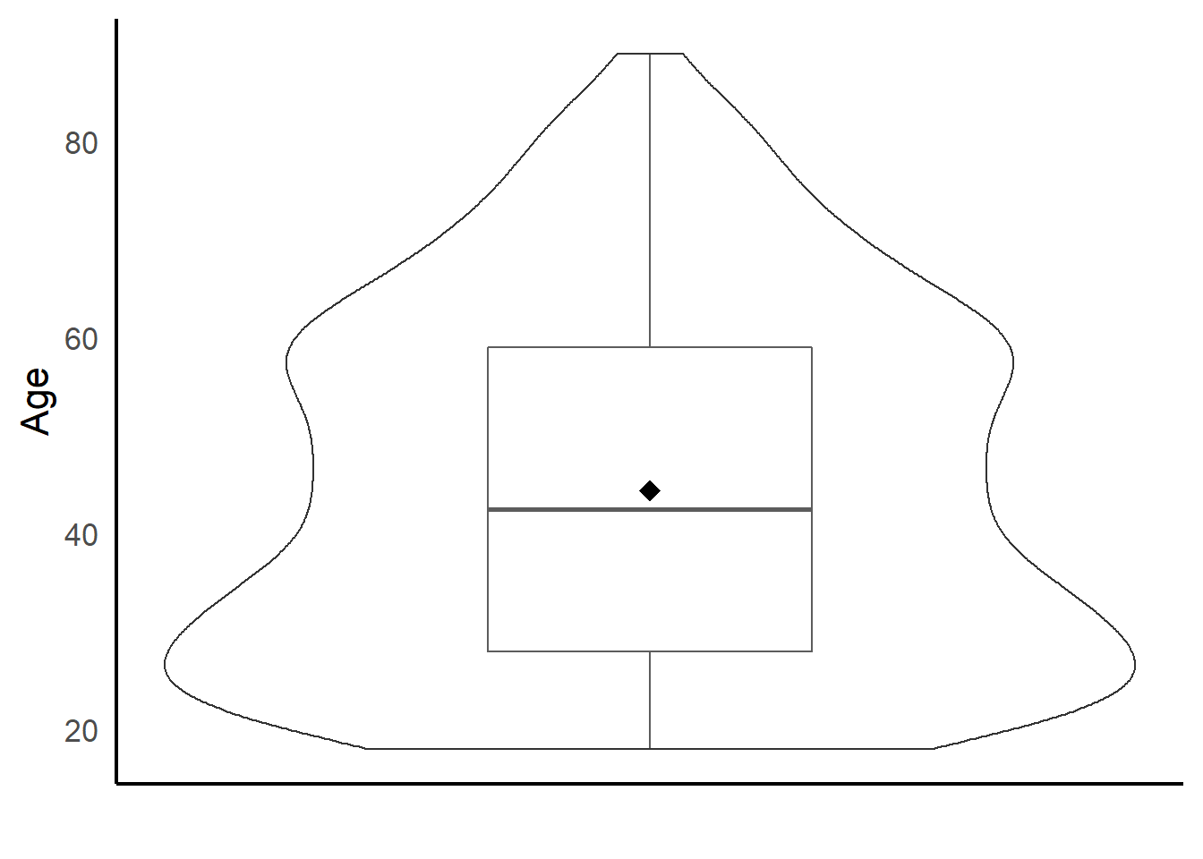

ggplot(depress, aes(y=CESD, x=1)) + 
  geom_boxplot(width=.3) + geom_violin(alpha=.2) +  
  ylab("CESD") + xlab("") + theme_classic(base_size = 16) + 
  geom_jitter(alpha=.3, width=.1) +
  theme(axis.ticks = element_blank(), axis.text.x = element_blank())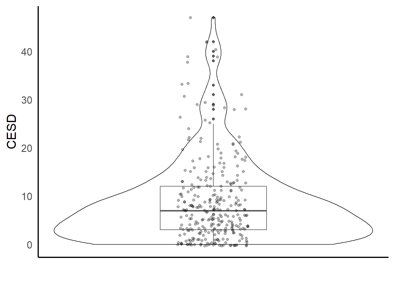

Bivariate

Categorical ~ Categorical

Two-way Frequency table

table(depress$gender, depress$educat) %>% kable()

	<HS	Some HS	HS Grad	Some college	BS	MS	PhD
Male	4	19	39	18	17	8	6
Female	1	42	75	30	26	6	3

Two-way cell proportions

kable(
  addmargins(
    prop.table(table(depress$gender, depress$educat))*100
    ),
  digits=1)

	<HS	Some HS	HS Grad	Some college	BS	MS	PhD	Sum
Male	1.4	6.5	13.3	6.1	5.8	2.7	2.0	37.8
Female	0.3	14.3	25.5	10.2	8.8	2.0	1.0	62.2
Sum	1.7	20.7	38.8	16.3	14.6	4.8	3.1	100.0

Two-way row proportions

kable(
  addmargins(
    prop.table(table(depress$gender, depress$educat), margin=1)*100
  ),
  digits=1)

	<HS	Some HS	HS Grad	Some college	BS	MS	PhD	Sum
Male	3.6	17.1	35.1	16.2	15.3	7.2	5.4	100
Female	0.5	23.0	41.0	16.4	14.2	3.3	1.6	100
Sum	4.2	40.1	76.1	32.6	29.5	10.5	7.0	200

Two-way column proportions

kable(
  addmargins(
    prop.table(table(depress$gender, depress$educat), margin=2)*100
  ),
  digits=1)

	<HS	Some HS	HS Grad	Some college	BS	MS	PhD	Sum
Male	80	31.1	34.2	37.5	39.5	57.1	66.7	346.2
Female	20	68.9	65.8	62.5	60.5	42.9	33.3	353.8
Sum	100	100.0	100.0	100.0	100.0	100.0	100.0	700.0

Bivariate stacked barchart

phna <- parhiv %>% select(JOBMO, EDUMO) %>% na.omit()
pct.cc <- biv.n.col.p(phna, "EDUMO", "JOBMO")

ggplot(phna, aes(x=EDUMO, fill=JOBMO)) + 
  geom_bar() + 
  theme_classic(base_size = 16) + 
  scale_fill_grey(name="Job Status") + xlab("") + 
  theme(legend.position="top", legend.title=element_text(size=10), legend.text=element_text(size=10)) +
  coord_equal(1/30) + ylab("Frequency") + 
  scale_x_discrete(labels = function(x) lapply(strwrap(x, width = 12, simplify = FALSE), 
                                               paste, collapse="\n")) + 
  theme(axis.ticks.x=element_blank())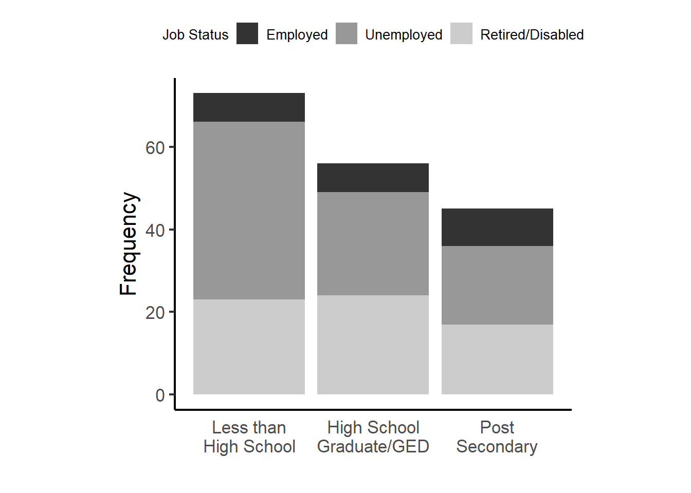

Bivariate stacked barchart

ggplot(pct.cc, aes(x=EDUMO, fill=JOBMO)) + 
  geom_bar(aes(y=pct), stat='identity') + 
  scale_fill_grey(guide=FALSE) + 
  theme_classic(base_size = 16) + 
  xlab("") + ylab("Percent") + 
  scale_y_continuous(labels=percent) + 
  coord_equal(1/0.35) + 
  scale_x_discrete(labels = function(x) lapply(strwrap(x, width = 12, simplify = FALSE), 
                                               paste, collapse="\n")) + 
  theme(axis.ticks.x=element_blank())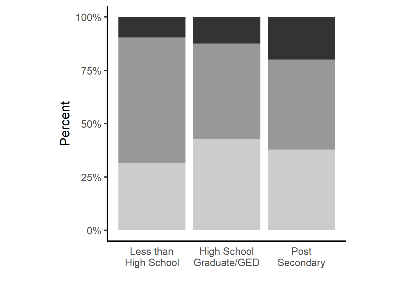

Bivariate side by side barchart

ggplot(pct.cc, aes(x=EDUMO, y=pct, fill=JOBMO)) + 
  scale_fill_grey(name="Job Status") + 
  geom_bar(stat="identity", position = "dodge") +  
  theme_classic(base_size = 16) + xlab("") + 
  scale_y_continuous(labels = percent) + 
  ylab("Percent") + 
  scale_x_discrete(labels = function(x) lapply(strwrap(x, width = 12, simplify = FALSE), 
                                               paste, collapse="\n")) + 
  theme(axis.ticks.x=element_blank())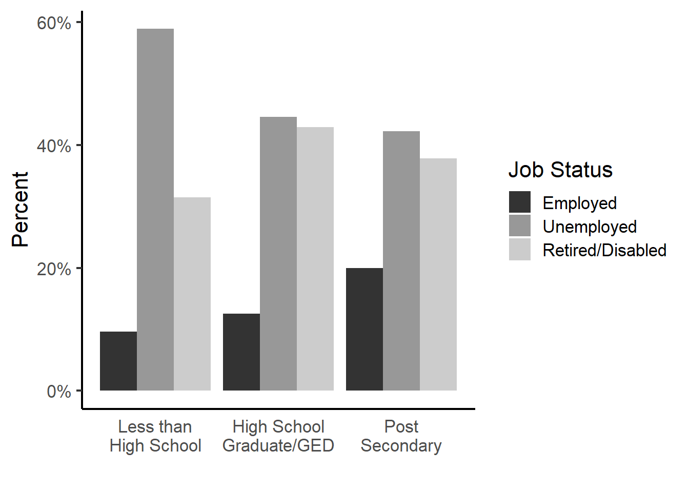

Bivariate dot plot for differences

ggplot(pct.cc, aes(x=count, y=reorder(JOBMO, count))) + 
  geom_point(size = 3) + 
  xlab("Frequency") + 
  facet_grid(EDUMO ~ ., labeller=label_wrap_gen(14)) +
  geom_segment(aes(yend=JOBMO), xend=0, color='grey50') + 
  ylab("Job Status") + theme_bw(base_size = 16) +
  theme(panel.grid.major.y = element_blank())  + 
  theme(axis.ticks.y=element_blank())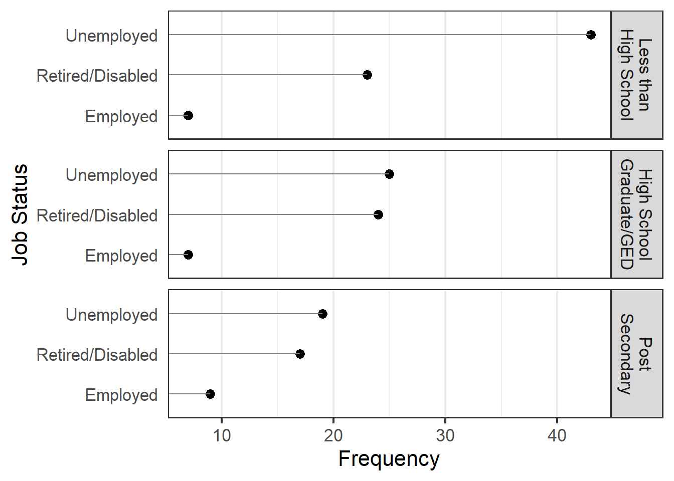

Bivariate dot plot for differences

bdpd <- parhiv %>% mutate(gender=factor(GENDER, labels=c("Male", "Female"))) %>% 
           select(JOBMO, gender) %>% na.omit() %>% 
           group_by(JOBMO, gender) %>% 
           summarise(count=n())

ggplot(bdpd, aes(x=count, y=reorder(JOBMO, count))) + 
              geom_point(aes(shape=gender), size=3) + 
              geom_line(aes(group=JOBMO)) +
  scale_shape_discrete(name="Gender of \n teen") +
  xlab("Frequency") + 
  ylab("Mother's Job Status") + 
  theme_bw(base_size = 16) +
  theme(panel.grid.major.y = element_blank())  + 
  theme(axis.ticks.y=element_blank())

Mosaic Plot

kable(
  prop.table(
    table(phna$EDUMO, phna$JOBMO)
    )*100, 
  digits=1)

	Employed	Unemployed	Retired/Disabled
Less than High School	4.0	24.7	13.2
High School Graduate/GED	4.0	14.4	13.8
Post Secondary	5.2	10.9	9.8

varnames <- list(set_varnames=c(JOBMO="Job Status", EDUMO="Highest Education Level"), 
                 rot_labels = c(0,90,0,0),
                 offset_varnames = c(left = 5, top=1), 
                 just_labels=c(left="right"))
lnames <- list(EDUMO = c("Less than\nHigh School", "High School\nGraduate/GED", "Post\nSecondary"))

mosaic(JOBMO~EDUMO, data=phna, color=TRUE, 
    set_labels=lnames,
    labeling_args = varnames,  
    margins=c(top=5, right=0, left=7))

Continuous ~ Continuous

Scatterplot

ggplot(depress, aes(x=AGE, y=CESD)) + geom_point(size=1, col="grey") + theme_classic(base_size = 16) +  
  xlab("Age") + ylab("CESD") + 
  geom_smooth(se=FALSE, method="lm", color="black", aes(linetype="Linear"))+ 
  geom_smooth(se=FALSE, method="loess", color="black", aes(linetype="Lowess"))+ 
  scale_linetype_manual(values = c("solid","dashed"), name="line types",
                        labels=c("Linear","Lowess"),guide="legend")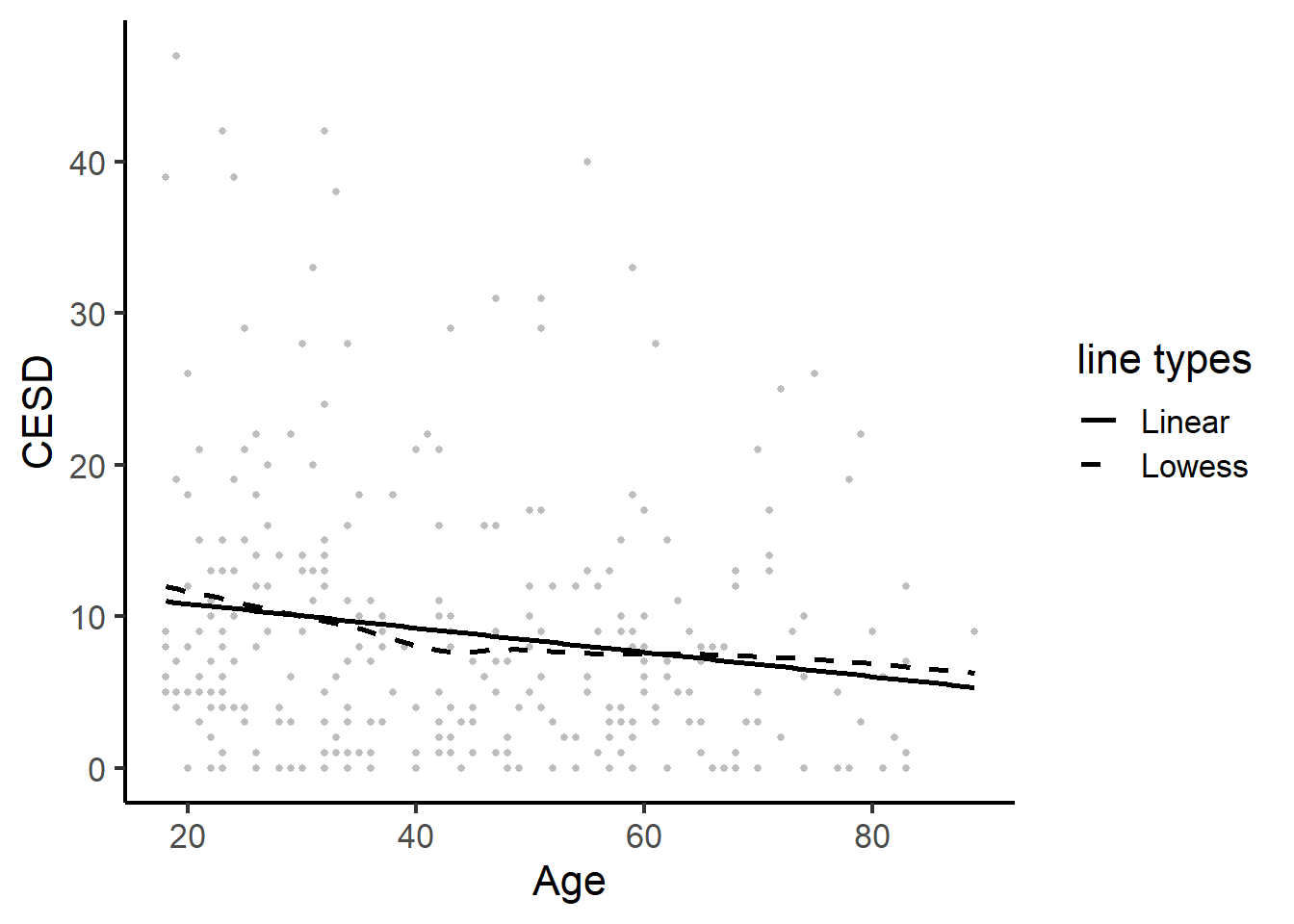

Profile plot

ggplot(mice, aes(y=WEIGHT, x=DAY, group=ID)) + 
  geom_point() + geom_line() + 
  theme_classic(base_size = 16) + 
  ylab("Weight (g)") + xlab("Time (Days)")

Bivariate Continuous + Categorical

ggplot(depress, aes(y=CESD, x=gender, color=gender)) +
  scale_color_grey(start=0, end=0.5,guide=FALSE) +
  geom_boxplot(width=.3) + geom_violin(alpha=.2) +  
  ylab("CESD") + xlab("") + 
  theme_classic(base_size = 20) + 
  stat_summary(fun.y=mean, geom="point", shape=18, size=4)  + 
  theme(axis.ticks.x=element_blank())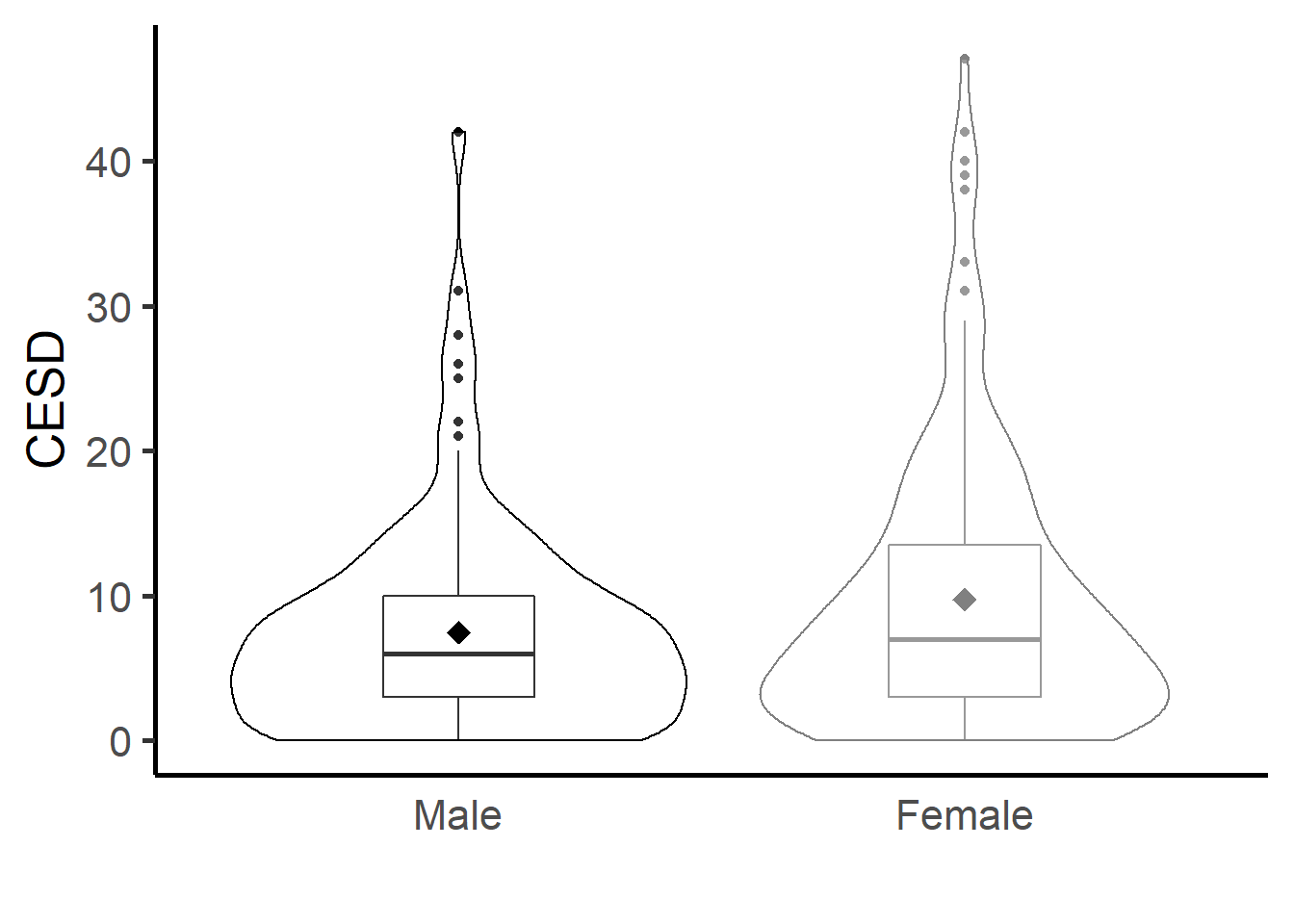

ggplot(depress, aes(x=CESD, color=gender)) + 
  geom_density() + theme_classic(base_size = 20) + 
  ylab("Density") + xlab("CESD")+
  scale_color_grey(start=0, end=0.5)+
  theme(axis.ticks = element_blank(), axis.text.y = element_blank()) + 
  theme(legend.justification=c(1,1), legend.position=c(1,1))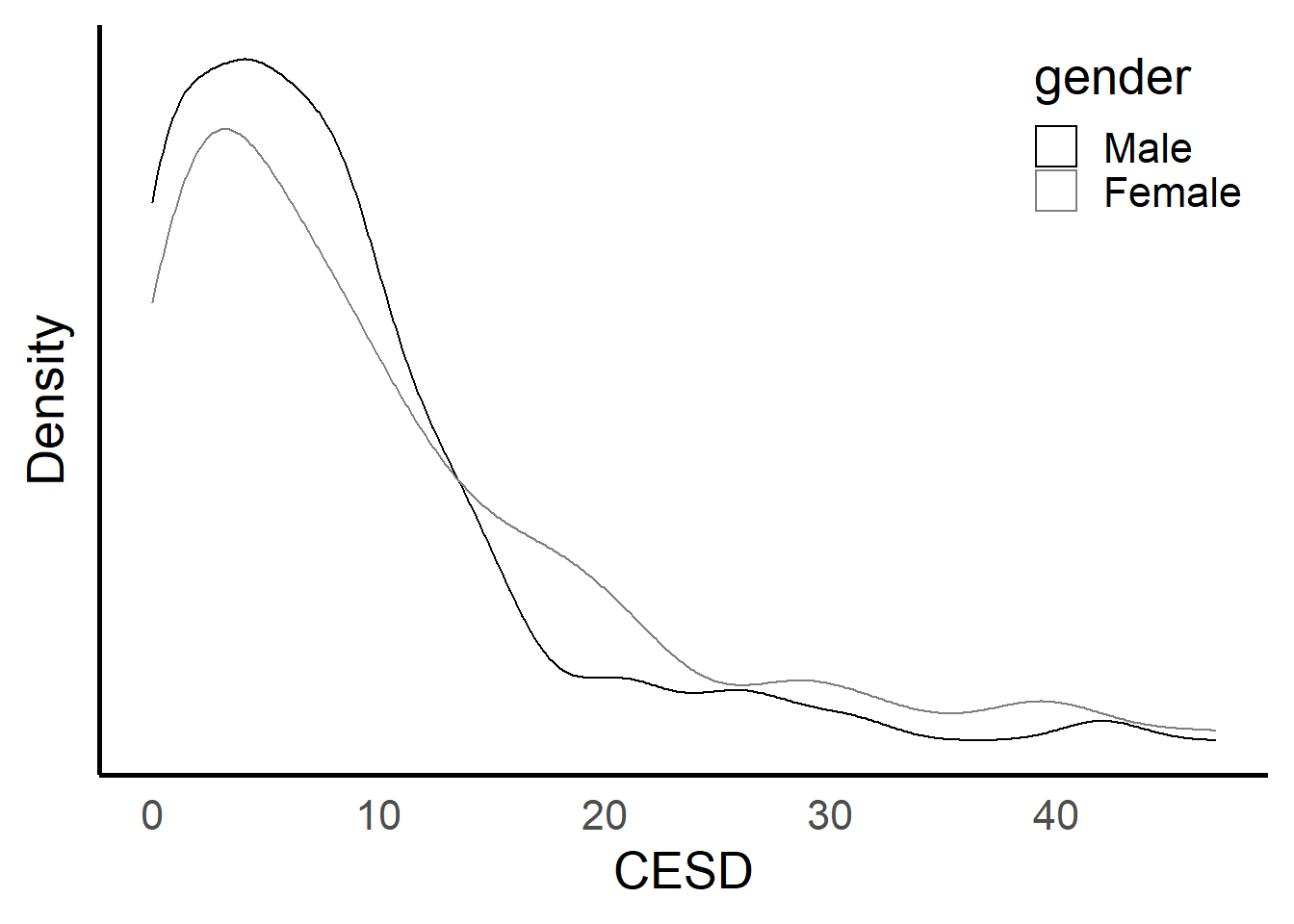

ggplot(depress, aes(x=CESD, fill=gender)) +  
  facet_grid(gender ~ .) + 
  xlab("CESD")+ylab("Frequency") + 
  geom_histogram() + theme_bw(base_size = 20) + 
  scale_fill_grey(start=0, end=0.5,guide=FALSE) +
  theme(axis.ticks = element_blank(), axis.text.y = element_blank()) + 
  theme(legend.justification=c(1,1), legend.position=c(1,1))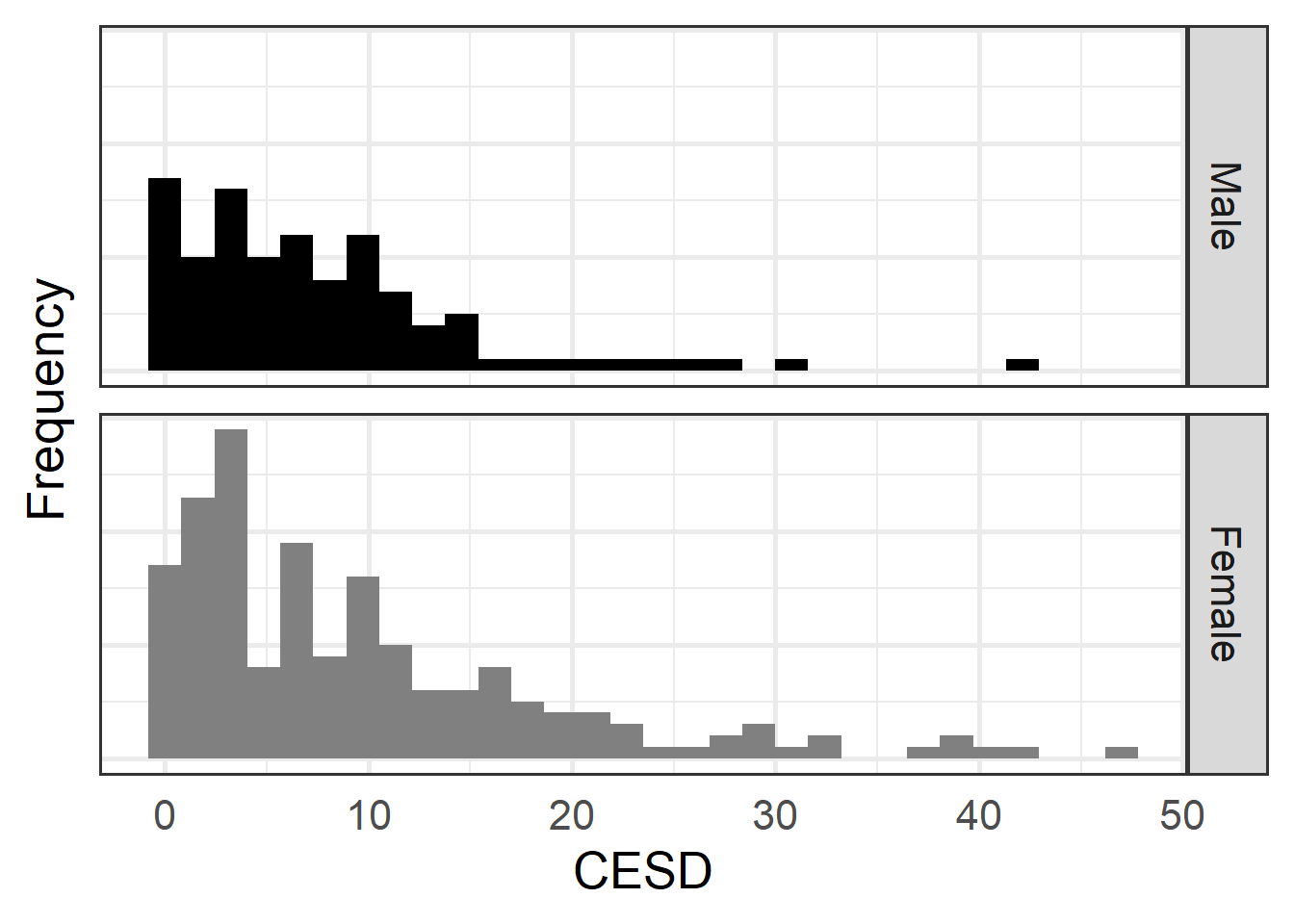

Multivariate

Scatterplots

ggplot(depress, aes(x=AGE, y=CESD, color=gender)) + 
  scale_color_grey() + 
  geom_point() +  
  theme_classic(base_size = 20) + 
  xlab("Age") + ylab("CESD")

ggplot(depress, aes(x=AGE, y=CESD, shape=gender)) + 
  geom_point() +  
  theme_classic(base_size = 20) + 
  xlab("Age") + ylab("CESD")

ggplot(depress, aes(x=AGE, y=CESD, size=INCOME)) + 
  geom_point(shape=21) + 
  theme_classic(base_size = 20) + 
  xlab("Age") + ylab("CESD") + 
  scale_size_continuous(limits=c(0,70), breaks = seq(0,70,by=10))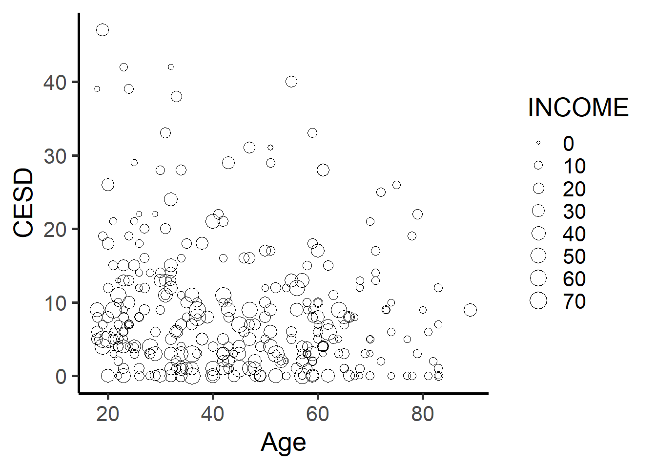

ggplot(depress, aes(x=AGE, y=CESD, fill=INCOME)) + 
  geom_point(shape=21, size=5) +
  theme_classic(base_size = 20) + 
  xlab("Age") + ylab("CESD") + 
  scale_fill_gradient(low="white", high="black")

Hist panel

ggplot(filter(parhiv, !is.na(EDUMO) & !is.na(JOBMO)), aes(x=bsi_overall)) +  
  ylab("Frequency") + 
  geom_histogram()+  
  facet_grid(EDUMO~JOBMO, labeller=label_wrap_gen(14)) +
  scale_y_continuous(breaks=seq(0,10,by=2))+
  theme_bw(base_size = 18) +
  xlab("Overall BSI score")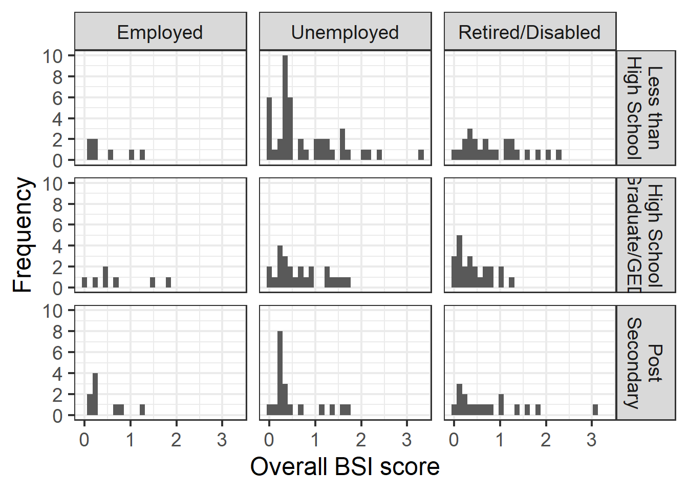

Scatterplot matrix

library(psych)
c.vars <- parhiv[,c("bsi_overall", "parent_bonding", 'AGESMOKE', 'AGEALC')]
names(c.vars) <- c("BSI", "Parental care subscale", "Age started smoking", "Age started drinking")

pairs.panels(c.vars, hist.col="grey80", col=1, rug=FALSE, cex.cor = .5, ellipses = FALSE)

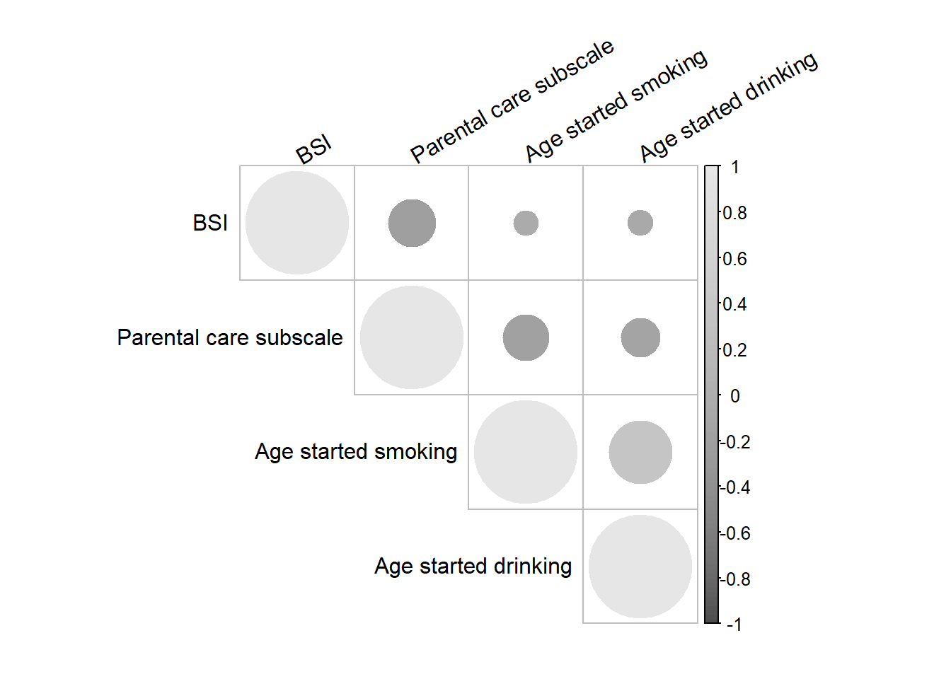
Correlation plot

library(corrplot)

corrplot(cor(c.vars, use='pairwise.complete.obs'), type="upper", col=gray.colors(100), 
         tl.col="black", tl.srt=30)

Chapter 04: Data Visualization

Robin Donatello

Last update 2021-08-07

Load Libraries

Helper functions

Load & prepare data

Demo

Univariate

Categorical

Univariate barplot with counts

Univariate barplot with percentages

Cleveland Dotplot

Pie Chart

Stem-leaf plot

Stripchart

Continuous

Univariate histogram

Univariate histogram with default bins

Univariate Density

Univariate boxplot

Univariate boxplot modified

Univariate boxplot

Bivariate

Categorical ~ Categorical

Two-way Frequency table

Two-way cell proportions

Two-way row proportions

Two-way column proportions

Bivariate stacked barchart

Bivariate stacked barchart

Bivariate side by side barchart

Bivariate dot plot for differences

Bivariate dot plot for differences

Mosaic Plot

Continuous ~ Continuous

Scatterplot

Profile plot

Bivariate Continuous + Categorical

Multivariate

Scatterplots

Hist panel

Scatterplot matrix

Correlation plot